|
Visual Servoing Platform
version 3.6.1 under development (2024-04-26)
|
|
Visual Servoing Platform
version 3.6.1 under development (2024-04-26)
|
ViSP allows simultaneously the tracking of a markerless object using the knowledge of its CAD model while providing its 3D localization (i.e., the object pose expressed in the camera frame) when a calibrated camera is used [8], [47]. Considered objects should be modeled by lines, circles or cylinders. The CAD model of the object could be defined in vrml format (except for circles), or in cao format (a home-made format).
This tutorial focuses on vpMbGenericTracker class that was introduced in ViSP 3.1.0. This class brings a generic way to consider different kind of visual features used as measures by the model-based tracker and allows also to consider either a single camera or multiple cameras observing the object to track. This class replaces advantageously the usage of the following classes vpMbEdgeTracker, vpMbKltTracker or the one mixing edges and keypoints vpMbEdgeKltTracker that will continue to exist in ViSP but that we don't recommend to use, since switching from one class to an other may be laborious. If for one reason or another you still want to use these classes, we invite you to follow Tutorial: Markerless model-based tracking (deprecated).
In this tutorial, we will show how to use vpMbGenericTracker class in order to track an object from images acquires by a monocular color camera using either moving edges, either keypoints, or either a combination of them using an hybrid scheme. To illustrate this tutorial we will consider that the object to track is a tea box.
Note that all the material (source code, input video, CAD model) described in this tutorial is part of ViSP source code (in tracking/model-based/generic folder) and could be found in https://github.com/lagadic/visp/tree/master/tracking/model-based/generic.
Considering the use case of a monocular color camera, the tracker implemented in vpMbGenericTracker class allows to consider a combination of the following visual features:
The moving-edges and KLT features require a RGB camera but note that these features operate on grayscale image.
Note also that combining the visual features (moving edges + keypoints) can be a good way to improve the tracking robustness.
Depending on your use case the following optional third-parties may be used by the tracker. Make sure ViSP was build with the appropriate 3rd parties:
OpenCV: Essential if you want to use the keypoints as visual features that are detected and tracked thanks to the KLT tracker. This 3rd party may be also useful to consider input videos (mpeg, png, jpeg...).Ogre 3D: This 3rd party is optional and could be difficult to install on OSX and Windows. To begin with the tracker we don't recommend to install it. Ogre 3D allows to enable Advanced visibility via Ogre3D.Coin 3D: This 3rd party is also optional and difficult to install. That's why we don't recommend to install Coin 3D to begin with the tracker. Coin 3D allows only to consider CAD model in wrml format instead of the home-made CAD model in cao format.For classical features working on grayscale image, you have to use the following data type:
You can convert to a grayscale image if the image acquired is in RGBa data type:
Since ViSP 3.2.1, it is also possible to consider color images as input with the following data type:
To start with the generic markerless model-based tracker we recommend to understand the tutorial-mb-generic-tracker.cpp source code that is given and explained below.
The tutorial-mb-generic-tracker.cpp example uses the following data as input:
teabox.mpg is the default video.teabox.cao is the default one. See Tracker CAD model section to learn how the teabox is modeled and section CAD model in cao format to learn how to model an other object.*.init that contains the 3D coordinates of some points used to compute an initial pose which serves to initialize the tracker. The user has than to click in the image on the corresponding 2D points. The default file is named teabox.init. The content of this file is detailed in Initialization by user click section.*.ppm that may help the user to remember the location of the corresponding 3D points specified in *.init file. To know more about this file see Initialization by user click section.As an output the tracker provides the pose  corresponding to a 4 by 4 matrix that corresponds to the geometric transformation between the frame attached to the object (in our case the tea box) and the frame attached to the camera. The pose is return as a vpHomogeneousMatrix container.
The following example that comes from tutorial-mb-generic-tracker.cpp allows to track a tea box modeled in cao format using either moving edges of keypoints as visual features.
Once build, to see the options that are available in the previous source code, just run:
By default, model/teabox/teabox.mpg video and model/teabox/teabox.cao model are used as input. Using "--tracker" option, you can specify which tracker has to be used:
"--tracker 0" to track only moving-edges:
"--tracker 1" to track only keypoints:
"--tracker 2" to track moving-edges and keypoints in an hybrid scheme:
With this example it is also possible to work on an other data set using "--video" and "--model" command line options. For example, if you run:
it means that the following images will be used as input:
and that in <path2> you have the following data:
myobject.init: The coordinates of at least four 3D points used for the initialization.myobject.cao: The CAD model of the object to track.myobject.ppm: An optional image that shows where the user has to click the points defined in myobject.init. Supported image format are png, ppm, png, jpeg.myobject.xml: An optional files that contains the tracker parameters that are specific to the image sequence and that contains also the camera intrinsic parameters obtained by calibration (see Tutorial: Camera intrinsic calibration). This file is handled in tutorial-mb-generic-tracker-full.cpp but not in tutorial-mb-generic-tracker.cpp. That's why since the video teabox.mpg was acquired by an other camera than yours, you have to set the camera intrinsic parameters in tutorial-mb-generic-tracker.cpp source code modifying the line: "--model ..." command line option.Hereafter is the description of the some lines introduced in the previous example.
First we include the header of the generic tracker.
The tracker uses image I and the intrinsic camera parameters cam as input.
As output, it estimates cMo, the pose of the object in the camera frame.
Once input image teabox.pgm is loaded in I, a window is created and initialized with image I. Then we create an instance of the tracker depending on "--tracker" command line option.
Then the corresponding tracker settings are initialized. More details are given in Tracker settings section.
Now we are ready to load the cad model of the object. ViSP supports cad model in cao format or in vrml format. The cao format is a particular format only supported by ViSP. It doesn't require an additional 3rd party rather then vrml format that require Coin 3rd party. We load the cad model in cao format from teabox.cao file which complete description is provided in teabox.cao example with:
It is also possible to modify the code to load the cad model in vrml format from teabox.wrl file described in teabox.wrl example. To this end modify the previous line with:
Once the model of the object to track is loaded, with the next line the display in the image window of additional drawings in overlay such as the moving edges positions, is then enabled by:
Now we have to initialize the tracker. With the next line we choose to use a user interaction (see Initialization by user click).
Next, in the infinite while loop, after displaying the next image, we track the object on a new image I.
The result of the tracking is a pose cMo that can be obtained by:
Next lines are used first to retrieve the camera parameters used by the tracker, then to display the visible part of the cad model using red lines with 2 as thickness, and finally to display the object frame at the estimated position cMo. Each axis of the frame are 0.025 meters long. Using vpColor::none indicates that x-axis is displayed in red, y-axis in green, while z-axis in blue. The thickness of the axis is 3.
The last lines are here to free the memory allocated for the display and tracker:
ViSP model-based tracker supports two different ways to describe CAD models, either in cao or in vrml format.
cao format is specific to ViSP. It allows to describe the CAD model of an object using a text file with extension .cao.vrml format is supported only if Coin 3rd party is installed. This format allows to describe the CAD model of an object using a text file with extension .wrl.To load a CAD model there is the vpMbGenericTracker::loadModel() function that could be used to load either cao model:
or a vrml model:
The content of the file teabox.cao used in the getting started Example source code but also in tutorial-mb-edge-tracker.cpp and in tutorial-mb-hybrid-tracker.cpp examples is given here:
This file describes the model of the tea box corresponding to the next image:
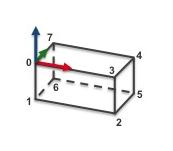
The tea box dimensions are the following:
We make the choice to describe the faces of the box from the 3D points that correspond to the vertices. We provide now a line by line description of the file. Notice that the characters after the '#' are considered as comments.
The content of the file teabox-triangle.cao used in the tutorial-mb-klt-tracker.cpp example is given here:
This file describes the model of the tea box corresponding to the next image:
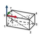
Until line 15, the content of this file is similar to the one described in teabox.cao example. Line 17 we specify that the model contains 12 faces. Each face is then described as a triangle.
The content of the teabox.wrl file used in tutorial-mb-generic-tracker-full.cpp and tutorial-mb-edge-tracker.cpp when teabox.cao is missing is given hereafter. This content is to make into relation with teabox.cao described in teabox.cao example. As for the cao format, teabox.wrl describes first the vertices of the box, then the edges that corresponds to the faces.
This file describes the model of the tea box corresponding to the next image:
We provide now a line by line description of the file where the faces of the box are defined from the vertices:
There are two ways to initialize the tracker, either by user interaction, either using an initial pose provided by a specific algorithm.
The tracker could be initialized by the user that has to click on at least 4 points on the object seen in the image. To this end, vpMbGenericTracker::initClick() function has to be used.
The previous line of code, loads a file named "<objectname>.init" and waits for user click. When an image named "<objectname>.ppm" exists besides "<objectname>.init" and when the last parameter of the function is set to true, the image is displayed to help the user to know where to click. Supported image formats are .ppm, .pgm, .png, .jpeg and .jpg.
Let us consider the teabox example.
The user has to click in the image on four vertices with their 3D coordinates defined in the "teabox.init" file. The following image "teabox.ppm" shows where the user has to click.
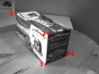
"teabox.ppm" used to help the user to initialize the tracker.Matched 2D and 3D coordinates are then used to compute an initial pose used to initialize the tracker. Note also that the third optional argument "true" is used here to enable the display of an image that may help the user for the initialization. The name of this image is the same as the "*.init" file except the extension that should be ".ppm". In our case it will be "teabox.ppm".
The content of teabox.init file that defines 3D coordinates of some points of the model used during user initialization is provided hereafter. Note that all the characters after character '#' are considered as comments.
We give now the signification of each line of this file:
Here the user has to click on vertex 0, 3, 2 and 5 in the window that displays image I. From the 3D coordinates defined in teabox.init and the corresponding 2D coordinates of the vertices obtained by user interaction a pose is computed that is then used to initialize the tracker.
How to choose good points for manual initialization
To select which 3D points to put in the .init file that are used to initialize manually the tracker, you should ensure that:
.init file) in the image must be visible.cao file.The other way to initialize the tracker is to use an initial pose provided by an external algorithm. To this end, vpMbGenericTracker::initFromPose() function has to be used.
Initial pose named cMo is here a vpHomogeneousMatrix object.
There are several ways to get an initial pose:
Instead of setting the tracker parameters from source code, it is possible to specify the settings from an XML file. As done in tutorial-mb-generic-tracker-full.cpp example, to read the parameters from an XML file, simply modify the code like:
The content of the XML file teabox.xml that is considered by default is the following:
Depending on the visual features that are used all the XML tags are not useful:
<ecm> tag corresponds to the moving-edges settings<klt> tag corresponds to the keypoint visual features and especially the KLT tracker settings used to detect and track the keypoints<camera> tag is used to define the camera intrinsic parameters<face> tag is used by the visibility algorithm used to determine if a face of the object is visible or not.Moving-edges settings affect the way the visible edges of an object are tracked. These settings could be tuned either from XML using <ecm> tag as:
of from source code using vpMbGenericTracker::setMovingEdge() method:
Either from xml or from the previous source code you can set:
<mask>/<size> xml tag, you will define the size of the convolution mask used to detect an edge. Possible values are 3, 5 or 7. We recommend to use 5.<mask>/<nb_mask> xml tag, you will set the number of mask applied to determine the object contour. The number of mask determines the precision of the normal of the edge for every sample. If precision is 2 deg, then there are 360/2 = 180 masks. Recommended value is 180.<range>/<tracking> xml tag, you will define the range on both sides of the reference pixel along the normal of the contour used to track a moving-edge. If the displacement of the tracked object in two successive images is large, you have to increase this parameter.<contrast>/<edge_threshold_type> xml tag, you will define the type of likelihood threshold used to determined if the moving edge is valid or not. Two values are possible: vpMe::OLD_THRESHOLD corresponding to 0, or vpMe::NORMALIZED_THRESHOLD corresponding to a value of 1 in the xml file. To keep compatibility with previous ViSP releases, the default type is set to vpMe::OLD_THRESHOLD in vpMe constructor, but we recommend to use the normalized threshold.<contrast>/<edge_threshold> xml tag, you will define the likelihood threshold used to determined if the moving edge is valid or not.Remmember that the value should be always in [0 ; 255].
<contrast>/<mu1> xml tag, you will define the minimum image contrast allowed to detect a contour. We recommend to keep this value to 0.5.<contrast>/<mu2> xml tag, you will define the maximum image contrast allowed to detect a contour. We recommend to keep this value to 0.5.<sample>/<step> xml tag, you will define the minimum distance in pixel between two discretized moving-edges. To increase the number of moving-edges you have to reduce this parameter.Keypoint settings affect tracking of keypoints on visible faces using KLT. These settings could be tuned either from XML using <klt> tag as:
of from source code using vpMbKltTracker::setKltOpencv() and vpMbKltTracker::setMaskBorder() methods:
With the previous parameters you can set:
<klt>/<mask_border> xml tag, you can specify the size of the mask corresponding to a zone inside the face along the contour in which the keypoints will not be detected. A mask size of zero means that keypoints can be detected on the contour.<klt>/<max_features> xml tag, you can set the maximum number of keypoint features to track in the image.<klt>/<window_size> xml tag, you can set the window size used to refine the corner locations.<klt>/<quality> xml tag, you can set the parameter characterizing the minimal accepted quality of image corners. Corners with quality measure less than this parameter are rejected. This means that if you want to have more keypoints on a face, you have to reduce this parameter.<klt>/<min_distance> xml tag, you can set the minimal Euclidean distance between detected corners during keypoint detection stage used to initialize keypoint location.<klt>/<harris> xml tag, you can set the free parameter of the Harris detector.<klt>/<size_block> xml tag, you can set the size of the averaging block used to track the keypoint features.<klt>/<pyramid_lvl> xml tag, you can set the maximal pyramid level. If the level is zero, then no pyramid is computed for the optical flow.Camera settings correspond to the intrinsic camera parameters without distortion. If images are acquired by a camera that has a large field of view that introduce distortion, images need to be undistorded before processed by the tracker. The camera parameters are then the one obtained on undistorded images.
Camera settings could be set from XML using <camera> tag as:
of from source code using vpMbTracker::setCameraParameters() method:
As described in vpCameraParameters class, these parameters correspond to  the ratio between the focal length and the size of a pixel, and
  the coordinates of the principal point in pixel.
An important setting concerns the visibility test that is used to determine if a face is visible or not. Note that moving-edges and keypoints are only tracked on visible faces. Three different visibility tests are implemented; with or without Ogre ray tracing and with or without scanline rendering. The default test is the one without Ogre and scanline. The functions vpMbTracker::setOgreVisibilityTest() and vpMbTracker::setScanLineVisibilityTest() allow to select which test to use.
Let us now highlight how the default visibility test works. As illustrated in the following figure, the angle  between the normal of the face and the line going from the camera to the center of gravity of the face is used to determine if the face is visible.
When no advanced visibility test is enable (we recall that this is the default behavior), the algorithm that computes the normal of the face is very simple. It makes the assumption that faces are convex and oriented counter clockwise. If we consider two parameters; the angle to determine if a face is appearing  , and the angle to determine if the face is disappearing
  , a face will be considered as visible if
 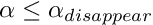 . We consider also that a new face is appearing if
 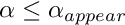 . These two parameters can be set either in the XML file:
or in the code:
Here the face is considered as appearing if  degrees, and disappearing if
  degrees.
The Ogre3D visibility test approach is based on ray tracing. When this test is enabled, the algorithm used to determine the visibility of a face performs (in addition to the previous test based on normals, i.e on the visible faces resulting from the previous test) another test which sets the faces that are partially occluded as non-visible. It can be enabled via:
When using the classical version of the ogre visibility test (which is the default behavior when activating this test), only one ray is used per polygon to test its visibility. As shown on the figure above, this only ray is sent from the camera to the center of gravity of the considered polygon. If the ray intersects another polygon before the considered one, it is set as non-visible. Intersections are computed between the ray and the axis-aligned bounding-box (AABB) of each polygon. In the figure above, the ray associated to the first polygon intersects first the AABB of the second polygon so it is considered as occluded. As a result, only the second polygon will be used during the tracking phase. This means that when using the edges, only the blue lines will be taken into account, and when using the keypoints, they will be detected only inside the second polygon (blue area).
Additionally, it is also possible to use a statistical approach during the ray tracing phase in order to improve the visibility results.
Contrary to the classical version of this test, the statistical approach uses multiple rays per polygons (4 in the example above). Each ray is sent randomly toward the considered polygon. If a specified ratio of rays do not have intersected another polygon before the considered one, the polygon is set as visible. In the example above, three ray on four return the first polygon as visible. As the ratio of good matches is more than 70% (which corresponds to the chosen ratio in this example) the first polygon is considered as visible, as well as the second one. As a result, all visible blue lines will be taken into account during the tracking phase of the edges and the keypoints that are detected inside the green area will be also used. Unfortunately, this approach is a polygon based approach so the dashed blue lines, that are not visible, will also be used during the tracking phase. Plus, keypoints that are detected inside the overlapping area won't be well associated and can disturb the algorithm.
Contrary to the visibility test using Ogre3D, this method does not require any additional third-party library. As for the advanced visibility using Ogre3D, this test is applied in addition to the test based on normals (i.e on the faces set as visible during this test) and also in addition to the test with Ogre3D if it has been activated. This test is based on the scanline rendering algorithm and can be enabled via:
Even if this approach requires a bit more computing power, it is a pixel perfect visibility test. According to the camera point of view, polygons will be decomposed in order to consider only their visible parts. As a result, if we consider the example above, dashed red lines won't be considered during the tracking phase and detected keypoints will be correctly matched with the closest (in term of depth from the camera position) polygon.
Additionally to the visibility test described above, it is also possible to use clipping. Firstly, the algorithm removes the faces that are not visible, according to the visibility test used, then it will also remove the faces or parts of the faces that are out of the clipping planes. As illustrated in the following figure, different clipping planes can be enabled.
Let us consider two plane categories: the ones belonging to the field of view or FOV (Left, Right, Up and Down), and the Near and Far clipping planes. The FOV planes can be enabled by:
which is equivalent to:
Of course, if the user just wants to activate Right and Up clipping, he will use:
For the Near and Far clipping it is quite different. Indeed, those planes require clipping distances. Here there are two choices, either the user uses default values and activate them with:
or the user can specify the distances in meters, which will automatically activate the clipping for those planes:
It is also possible to enable them in the XML file. This is done with the following lines:
Here for simplicity, the user just has the possibility to either activate all the FOV clipping planes or none of them (fov_clipping requires a boolean).
The first way to detect a tracking failure is to catch potential internal exceptions returned by the tracker:
If you are using edges as features, you can exploit the internal tracker state using vpMbTracker::getProjectionError() to get a scalar criteria between 0 and 90 degrees corresponding to the cad model projection error. This criteria corresponds to the mean angle between the gradient direction of the moving-edges features that are tracked and the normal of the projected cad model. Thresholding this scalar allows to detect a tracking failure. Usually we consider that a projection angle higher to 25 degrees corresponds to a tracking failure. This threshold needs to be adapted to your setup and illumination conditions.
When edges are not tracked, meaning that your tracker uses rather klt keypoints or depth features, there is vpMbGenericTracker::computeCurrentProjectionError() function that may be useful.
Tracking failure detection is used in tutorial-mb-generic-tracker-live.cpp and tutorial-mb-generic-tracker-rgbd-realsense.cpp examples.
The model-based tracker can also update a covariance matrix corresponding to the estimated pose. But from our experience, analysing the diagonal of the 6 by 6 covariance matrix doesn't allow to detect a tracking failure. If you want to have a trial, we recall the way to get the covariance matrix:
The following code shows how to access to the CAD model
The level of detail (LOD) consists in introducing additional constraints to the visibility check to determine if the features of a face have to be tracked or not. Two parameters are used:
The tracker allows to enable/disable the level of detail concept using vpMbTracker::setLod() function. This example permits to set LOD settings to all elements :
This example permits to set LOD settings to specific elements denominated by his name.
Furthermore, to set a name to a face see How to set a name to a face.
The first thing to do is to declare the differents points. Then you define each segment of the face with the index of the start point and with the index of the end point. Finally, you define the face with the index of the segments which constitute the face.
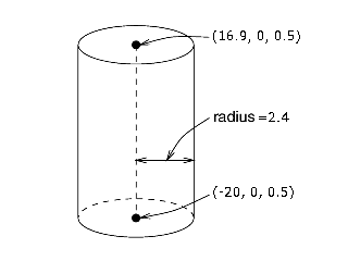
The first thing to do is to declare the two points defining the cylinder axis of revolution. Then you declare the cylinder with the index of the points that define the cylinder axis of revolution and with the cylinder radius.
The first thing to do is to declare three points: one point for the center of the circle and two points on the circle plane (i.e. not necessary located on the perimeter of the circle but on the plane of the circle). Then you declare your circle with the radius and with index of the three points.
By default, the cMo pose estimated by the tracker corresponds to the homogeneous transformation between the camera frame and the CAD model object frame. The tracker can consider an optional transformation matrix (currently only for .cao) to transform 3D points of the CAD model expressed in the original object frame to a desired object frame. Let us call this matrix oMod. When this matrix is introduced, the tracker estimates the homogeneous transformation between the camera and the modified CAD model object frame.
The tracker has the ability to modify the location of the CAD model origin frame, introducing an extra homogeneous transformation. was designed to easily modify the location of the CAD model origin introducing an offset transformation matrix:
To load a CAD model there is the vpMbGenericTracker::loadModel() function that could be used to load either cao model:
It could be useful to define a complex model instead of using one big model file with all the declaration with different sub-models, each one representing a specific part of the complex model in a specific model file. To create a hierarchical model, the first step is to define all the elementary parts and then regroup them.
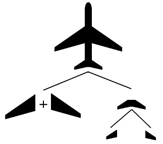
For example, if we want to have a model of a plane, we could represent as elementary parts the left and right wings, the tailplane (which is constituted of some other parts) and a cylinder for the plane fuselage. The following lines represent the top model of the plane.
To exploit the name of a face in the code, see sections about Level of detail (LOD) and How not to consider specific polygons.
It could be useful to give a name for a face in a model in order to easily modify his LOD parameters for example, or to decide if you want to use this face or not during the tracking phase. This is done directly in the .cao model file. For example, the next example shows how to set plane_fuselage as name for the cylinder used to model the plane fuselage and right reactor as name for the corresponding plane reactor modeled as a circle:
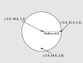
In ViSP 3.2.1 we introduce the capability to load a .cao model with 3D translation and rotation. For the translation, values are expressed in meters. For the rotation, the representation is the  axis-angle implemented in vpThetaUVector class. Values can be expressed in degrees or radians.
Let us model a square made with 4 lego 2x4 bricks as shown in the next immage.
Instead of modeling all the 4 brick, we can just model one brick and use translation and rotation to model the others.
The .cao model of the 2x4 brick located in ./lego_parts/brick-2x4.cao is the following:
Now to model a square made with 4 bricks, we can reuse the same 2x4 brick model introducing translation and rotation. The corresponding model ./lego-square.cao is the following:
The corresponding ./lego-square.init file could contain the following coordinates of the points
Now to see how to track this object you can jump to Test tracker on lego model with a live camera section.
As explained in section Level of detail (LOD) the parameters of the lod can be set in the source code. They can also be set directly in the configuration file or in the CAD model in cao format.
The following lines show the content of the configuration file :
In CAD model file, you can specify the LOD settings to the desired elements :
To exploit the name of a face in the code, see sections about Level of detail (LOD) and How not to consider specific polygons.
When using a wrml file, names are associated with shapes. In the example below (the model of a teabox), as only one shape is defined, all its faces will have the same name: "teabox_name".
When using model-based trackers, it is possible to not consider edge, keypoint or depth features tracking for specific faces. To do so, the faces you want to consider must have a name following How to set a name to a face.
If you want to enable (default behavior) or disable the edge tracking on specific face it can be done via:
If the boolean is set to false, the tracking of the edges of the faces that have the given name will be disable. If it is set to true (default behavior), it will be enable.
As for the edge tracking, the same functionality is also available when using keypoints via:
For the depth feature, this functionality is also available via:
or
The classical way to save tracking results is to use vpDisplay::getImage() as in tutorial-export-image.cpp to exploit the display window in order to get the image and all the drawings in overlay in a RGBa image and then to save the resulting image.
But on embedded systems, it is not always possible to open a display window with vpDisplayX, vpDisplayOpenCV or vpDisplayGDI to view real-time tracking results. That's why we propose to use vpMbGenericTracker::getModelForDisplay() and vpMbGenericTracker::getFeaturesForDisplay() in conjunction with vpImageDraw to draw tracking results directly in an image that could be saved during tracking.
The following code from testGenericTracker.cpp shows how to draw the CAD model in an image named resultsColor or resultsDepth:
There is also the possibility to draw the tracked features in the same images:
And then to save the images in a file:
By default the model-based tracker estimates the 6 degrees of freedom (dof) of the pose [tx, ty, tz, rx, ry, rz].
In the particular case where the model is a circle or a cylinder, the tracker does not consider the degree of freedom that it cannot estimate around the axis of symmetry or revolution of the object. Thus if the model consists of a circle of radius R defined in the plane  , the estimated degrees of freedom in the object frame correspond to [tx, ty, tz, rx, 0, rz] .
Given your use case it could be useful to reduce the number of dof to consider. For example, if your object is always parallel to the image plane, estimating only the translation can make the tracker more reliable. In this case, you can use the following code to avoid estimating the rotation.
Hereafter we provide the information to test the tracker with different objects.
Enter model-based tracker tutorial build folder:
There is tutorial-mb-generic-tracker-full binary that corresponds to the build of tutorial-mb-generic-tracker-full.cpp example. This example is an extension of tutorial-mb-generic-tracker.cpp that was explained in Getting started section.
to see the options that are available run:
By default all the parameters are set to work with the teabox example. Just run the binary without option:
You may also obtain the same results using:
In http://visp-doc.inria.fr/download/mbt-model/cubesat.zip you will find the model data set (.obj, .cao, .init, .xml, .ppm) and a video to test the CubeSAT object tracking. After unzip in a folder (let say /your-path-to-model) you may run the tracker with something similar to:
You should be able to obtain these kind of results:
In http://visp-doc.inria.fr/download/mbt-model/mmicro.zip you will find the model data set (.cao, .wrl, .init, .xml, .ppm) and a video to track the mmicro object. After unzip in a folder (let say $VISP_WS) you may run the tracker with something similar to:
You should be able to obtain these kind of results:
All the previous examples (teabox, CubeSAT, mmicro) were working with videos. We provide tutorial-mb-generic-tracker-live.cpp that allows to use a camera in order to test the tracker live.
This example tries to use the first grabber that is available in the following list:
By default, if you are on an Ubuntu like system that has libv4l-dev package installed, you should be able to grab images from a webcam without modifying the code.
To select an other grabber that corresponds to your camera you have to uncomment some lines at the beginning of tutorial-mb-generic-tracker-live.cpp tutorial:
For example to force the usage of vpRealSense2 class that allows to grab images from an Intel Realsense device like D435 or SR300, you should modify the code like:
Once modified, enter the build folder and build the tutorial:
Let us now consider the object made with 4 lego 2x4 bricks described in How to load cao model with transformation.
Once build, to get the usage, run:
To test the tracker on the lego-square object, run:
You should be able to obtain these kind of results:
Now if the tracker is working, you can learn the object running:
Once initialized by 4 user clicks, use the left click to learn on one or two images and then the right click to quit. In the terminal you should see printings like:
You can now use this learning to automize tracker initialization with:
If you run mbtEdgeTracking.cpp, mbtKltTracking.cpp or mbtEdgeKltTracking.cpp examples enabling Ogre visibility check (using "-o" option), you may encounter the following issue:
and then a wonderful runtime issue as in the next image:
It means maybe that Ogre version is not compatible with DirectX 11. This can be checked adding "-w" option to the command line:
Now the binary should open the Ogre configuration window where you have to select "OpenGL Rendering Subsystem" instead of "Direct3D11 Rendering Subsystem". Press then OK to continue and start the tracking of the cube.
This issue is similar to Model-based trackers examples are not working with Ogre visibility check. It may occur with tutorial-mb-edge-tracker.cpp, tutorial-mb-klt-tracker.cpp and tutorial-mb-hybrid-tracker.cpp. To make working the tutorials:
If you have a webcam, you are now ready to experiment the generic model-based tracker on a cube that has an AprilTag on one face following Tutorial: Markerless generic model-based tracking using AprilTag for.
There is also Tutorial: Object detection and localization to learn how to initialize the tracker without user click, by learning the object to track using keypoints when the object is textured. There is also Tutorial: Markerless generic model-based tracking using a stereo camera if you want to know how to extend the tracker to use a stereo camera or Tutorial: Markerless generic model-based tracking using a RGB-D camera if you want to extend the tracking by using depth as visual features. There is also this other Tutorial: Template tracking.