Unicycle with a fixed camera

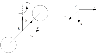
In this section we consider the following unicycle:

This robot has 2 dof: , the translational and rotational velocities that are applied at point E, considered as the end-effector. A camera is rigidly attached to the robot at point C. The homogeneous transformation between C and E is given by cMe. This transformation is constant.

The robot position evolves with respect to a world frame; wMe. When a new joint velocity is applied to the robot using setVelocity(), the position of the camera wrt the world frame is also updated; wMc.

To control the robot by visual servoing we need to introduce two visual features. If we consider a 3D point at position O as the target, to position the robot relative to the target we can consider the coordinate $x$ of the point in the image plane and , with the distance of point in the camera frame, as visual features. The first feature implemented in vpFeaturePoint allows to control , while the second one implemented in vpFeatureDepth . The position of the target in the world frame is given by wMo transformation. Thus the current visual feature ${\bf s} = (x, log(Z/Z^*))^\top$ and the desired feature ${\bf s}^* = (0, 0)^\top$ .

The code that does the simulation is provided in tutorial-simu-pioneer.cpp and given hereafter.

 
#include <iostream>
 
#include <visp3/core/vpConfig.h>
#include <visp3/core/vpHomogeneousMatrix.h>
#include <visp3/core/vpVelocityTwistMatrix.h>
#include <visp3/gui/vpPlot.h>
#include <visp3/robot/vpSimulatorPioneer.h>
#include <visp3/visual_features/vpFeatureBuilder.h>
#include <visp3/visual_features/vpFeatureDepth.h>
#include <visp3/visual_features/vpFeaturePoint.h>
#include <visp3/vs/vpServo.h>
 
int main()
{
#if defined(ENABLE_VISP_NAMESPACE)
  using namespace VISP_NAMESPACE_NAME;
#endif
  try {
    vpHomogeneousMatrix cdMo;
    cdMo[1][3] = 1.2;
    cdMo[2][3] = 0.5;
 
    vpHomogeneousMatrix cMo;
    cMo[0][3] = 0.3;
    cMo[1][3] = cdMo[1][3];
    cMo[2][3] = 1.;
    vpRotationMatrix cRo(0, atan2(cMo[0][3], cMo[1][3]), 0);
    cMo.insert(cRo);
 
    vpSimulatorPioneer robot;
    robot.setSamplingTime(0.04);
    vpHomogeneousMatrix wMc, wMo;
    robot.getPosition(wMc);
    wMo = wMc * cMo;
 
    vpPoint point(0, 0, 0);
    point.track(cMo);
 
    vpServo task;
    task.setServo(vpServo::EYEINHAND_L_cVe_eJe);
    task.setInteractionMatrixType(vpServo::DESIRED, vpServo::PSEUDO_INVERSE);
    task.setLambda(0.2);
    vpVelocityTwistMatrix cVe;
    cVe = robot.get_cVe();
    task.set_cVe(cVe);
 
    vpMatrix eJe;
    robot.get_eJe(eJe);
    task.set_eJe(eJe);
 
    vpFeaturePoint s_x, s_xd;
    vpFeatureBuilder::create(s_x, point);
    s_xd.buildFrom(0, 0, cdMo[2][3]);
    task.addFeature(s_x, s_xd, vpFeaturePoint::selectX());
 
    vpFeatureDepth s_Z, s_Zd;
    double Z = point.get_Z();
    double Zd = cdMo[2][3];
    s_Z.buildFrom(s_x.get_x(), s_x.get_y(), Z, log(Z / Zd));
    s_Zd.buildFrom(0, 0, Zd, 0);
    task.addFeature(s_Z, s_Zd);
 
#ifdef VISP_HAVE_DISPLAY
    // Create a window (800 by 500) at position (400, 10) with 3 graphics
    vpPlot graph(3, 800, 500, 400, 10, "Curves...");
 
    // Init the curve plotter
    graph.initGraph(0, 2);
    graph.initGraph(1, 2);
    graph.initGraph(2, 1);
    graph.setTitle(0, "Velocities");
    graph.setTitle(1, "Error s-s*");
    graph.setTitle(2, "Depth");
    graph.setLegend(0, 0, "vx");
    graph.setLegend(0, 1, "wz");
    graph.setLegend(1, 0, "x");
    graph.setLegend(1, 1, "log(Z/Z*)");
    graph.setLegend(2, 0, "Z");
#endif
 
    int iter = 0;
    for (;;) {
      robot.getPosition(wMc);
      cMo = wMc.inverse() * wMo;
 
      point.track(cMo);
 
      vpFeatureBuilder::create(s_x, point);
 
      Z = point.get_Z();
      s_Z.buildFrom(s_x.get_x(), s_x.get_y(), Z, log(Z / Zd));
 
      robot.get_cVe(cVe);
      task.set_cVe(cVe);
      robot.get_eJe(eJe);
      task.set_eJe(eJe);
 
      vpColVector v = task.computeControlLaw();
      robot.setVelocity(vpRobot::ARTICULAR_FRAME, v);
 
#ifdef VISP_HAVE_DISPLAY
      graph.plot(0, iter, v);               // plot velocities applied to the robot
      graph.plot(1, iter, task.getError()); // plot error vector
      graph.plot(2, 0, iter, Z);            // plot the depth
#endif
 
      iter++;
 
      if (task.getError().sumSquare() < 0.0001) {
        std::cout << "Reached a small error. We stop the loop... " << std::endl;
        break;
      }
    }
#ifdef VISP_HAVE_DISPLAY
    graph.saveData(0, "./v2.dat");
    graph.saveData(1, "./error2.dat");
 
    const char *legend = "Click to quit...";
    vpDisplay::displayText(graph.I, (int)graph.I.getHeight() - 60, (int)graph.I.getWidth() - 150, legend, vpColor::red);
    vpDisplay::flush(graph.I);
    vpDisplay::getClick(graph.I);
#endif
 
    // Kill the servo task
    task.print();
 
  }
  catch (const vpException &e) {
    std::cout << "Catch an exception: " << e << std::endl;
  }
}

We provide now a line by line explanation of the code.

Firstly we define cdMo the desired position the camera has to reach wrt the target. should be different from zero to be non singular. The camera has to keep a distance of 0.5 meter from the target.

vpHomogeneousMatrix cdMo ;
cdMo[1][3] = 1.2; // ty
cdMo[2][3] = 0.5; // tz

Secondly we specify cMo the initial position of the camera wrt the target.

vpHomogeneousMatrix cMo;
cMo[0][3] = 0.3;        // tx
cMo[1][3] = cdMo[1][3]; // ty
cMo[2][3] = 1.;         // tz
vpRotationMatrix cRo(0, atan2( cMo[0][3], cMo[1][3]), 0);
cMo.insert(cRo);

Thirdly by introducing our simulated robot we can compute the position of the target wMo and of the camera wMc wrt the world frame.

vpSimulatorPioneer robot ;
robot.setSamplingTime(0.04);
vpHomogeneousMatrix wMc, wMo;
robot.getPosition(wMc);
wMo = wMc * cMo;

Once all the frames are defined, we define a 3D point and its coordinates (0,0,0) in the object frame as the target.

vpPoint point;

point.setWorldCoordinates(0,0,0);

vpPoint::setWorldCoordinates

void setWorldCoordinates(double oX, double oY, double oZ)

Definition: vpPoint.cpp:111

We compute then its coordinates in the camera frame.

point.track(cMo);

vpForwardProjection::track

void track(const vpHomogeneousMatrix &cMo)

Definition: vpForwardProjection.cpp:102

A visual servo task is then instantiated.

vpServo task;

With the next line, we specify the king of visual servoing control law that will be used to control our mobile robot. Since the camera is mounted on the robot, we consider the case of an eye-in-hand visual servo. The robot controller provided in vpSimulatorPioneer allows to send velocities. This controller implements also the robot jacobian $\bf ^e J_e$ that links the end-effector velocity skew vector $\bf v_e$ to the control velocities . The also provided velocity twist matrix $\bf ^c V_e$ allows to transform a velocity skew vector expressed in the end-effector frame in the camera frame.

task.setServo(vpServo::EYEINHAND_L_cVe_eJe);

We specify then that the interaction matrix $\bf L$ is computed from the visual features at the desired position. The constant gain that allows an exponential decrease of the features error is set to 0.2.

task.setInteractionMatrixType(vpServo::DESIRED, vpServo::PSEUDO_INVERSE);

task.setLambda(0.2);

To resume, with the previous line, the following control law will be used:

$\left[\begin{array}{c} v_x \\ w_z \end{array}\right] = -0.2 \left( {\bf L_{s^*} {^c}V_e {^e}J_e}\right)^{+} ({\bf s} - {\bf s}^*)$

From the robot position we retrieve the velocity twist transformation $\bf ^c V_e$ that is then re-injected to the task.

vpVelocityTwistMatrix cVe;
cVe = robot.get_cVe();
task.set_cVe(cVe);

We do the same with the robot jacobian $\bf ^e J_e$ .

vpMatrix eJe;
robot.get_eJe(eJe);
task.set_eJe(eJe);

Let us now consider the visual features. We first instantiate the current and desired position of the 3D target point as a visual feature point.

vpFeaturePoint s_x, s_xd;

The current visual feature is directly computed from the perspective projection of the point position in the camera frame.

vpFeatureBuilder::create(s_x, point);

The desired position of the feature is set to (0,0). The depth of the point cdMo[2][3] is required to compute the feature position.

s_xd.buildFrom(0, 0, cdMo[2][3]);

Finally only the position of the feature along x is added to the task.

task.addFeature(s_x, s_xd, vpFeaturePoint::selectX());

We consider now the second visual feature that corresponds to the depth of the point. The current and desired features are instantiated with:

vpFeatureDepth s_Z, s_Zd;

Then, we get the current Z and desired Zd depth of the target.

double Z = point.get_Z();

double Zd = cdMo[2][3];

vpPoint::get_Z

double get_Z() const

Get the point cZ coordinate in the camera frame.

Definition: vpPoint.cpp:406

From these values, we are able to initialize the current depth feature:

s_Z.buildFrom(s_x.get_x(), s_x.get_y(), Z, log(Z/Zd));

and also the desired one:

s_Zd.buildFrom(0, 0, Zd, 0);

Finally, we add the feature to the task:

task.addFeature(s_Z, s_Zd);

Then comes the material used to plot in real-time the curves that shows the evolution of the velocities, the visual error and the estimation of the depth. The corresponding lines are not explained in this tutorial, but should be easily understand by reading Tutorial: Real-time curves plotter tool.

In the visual servo loop we retrieve the robot position and compute the new position of the camera wrt the target:

robot.getPosition(wMc) ;

cMo = wMc.inverse() * wMo;

We compute the coordinates of the point in the new camera frame:

point.track(cMo);

Based on these new coordinates, we update the point visual feature s_x:

vpFeatureBuilder::create(s_x, point);

and also the depth visual feature:

Z = point.get_Z() ;

s_Z.buildFrom(s_x.get_x(), s_x.get_y(), Z, log(Z/Zd)) ;

We also update the task with the values of the velocity twist matrix cVe and the robot jacobian eJe:

robot.get_cVe(cVe);
task.set_cVe(cVe);
robot.get_eJe(eJe);
task.set_eJe(eJe);

After all these updates, we are able to compute the control law:

vpColVector v = task.computeControlLaw();

Computed velocities are send to the robot:

robot.setVelocity(vpRobot::ARTICULAR_FRAME, v);

At the end, we stop the infinite loop when the visual error reaches a value that is considered as small enough:

if (task.getError().sumSquare() < 0.0001) {
  std::cout << "Reached a small error. We stop the loop... " << std::endl;
  break;
}

Unicycle with a moving camera

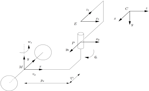
In this section we consider the following unicycle:

This robot has 3 dof: $(v_x, w_z, \dot q_{1})$ , as previously the translational and rotational velocities that are applied here at point M, and $\dot q_{1}$ the pan of the head. The position of the end-effector E depends on $q_{1}$ position. The camera at point C is attached to the robot at point E. The homogeneous transformation between C and E is given by cMe. This transformation is constant.

If we consider the same visual features than previously ${\bf s} = (x, log(Z/Z^*))^\top$ and the desired feature ${\bf s}^* = (0, 0)^\top$ , we are able to simulate this new robot simply by replacing vpSimulatorPioneer by vpSimulatorPioneerPan. The code is available in tutorial-simu-pioneer-pan.cpp.

You can just notice here that we compute the control law using the current interaction matrix; the one computed with the current visual feature values.

vpServo task;
task.setServo(vpServo::EYEINHAND_L_cVe_eJe);
task.setInteractionMatrixType(vpServo::CURRENT, vpServo::PSEUDO_INVERSE);

The following control law is used:

$\left[\begin{array}{c} v_x \\ w_z \\ \dot q_{1} \end{array}\right] = -0.2 \left( {\bf L_{s} {^c}V_e {^e}J_e}\right)^{+} ({\bf s} - {\bf s}^*)$

Next tutorial

You are now ready to see the next Tutorial: How to boost your visual servo control law.

Table of Contents

Unicycle with a fixed camera

Unicycle with a moving camera

Next tutorial