Introduction

We suppose that you are already familiar with the Tutorial: Using Particle Filter to filter your data.

The Particle Filters (PF) are a set of Monte Carlo algorithms that permit to approximate solutions for filtering problems even when the state-space and/or measurement space are non-linear.

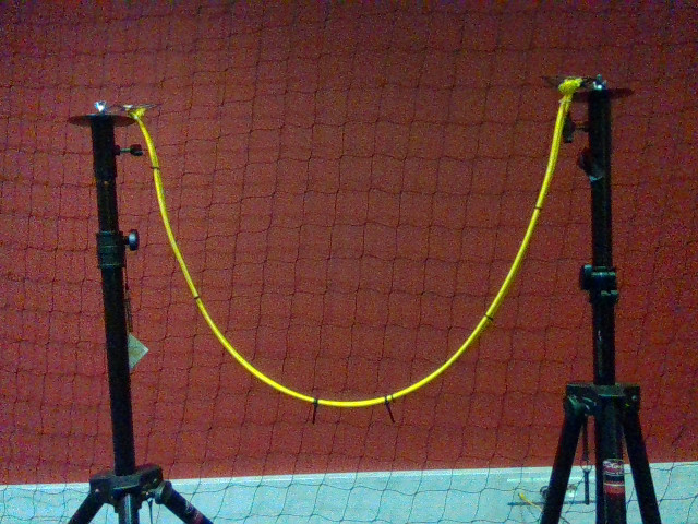
In this tutorial, we will use a PF to model a wire using polynomial interpolation . The PF is used to filter the noisy pixels in a segmented image in order to compute a model of the wire using polynomial interpolation. The color wire is observed by a static camera, in the following configuration:

The maths beyond the Particle Filter

The maths beyond the Particle Filter are explained in the documentation of the vpParticleFilter class. They are also explained in the The maths beyond the Particle Filter .

Explanations about the tutorial

The tutorial is split in three different programs:

tutorial-pf-curve-fitting-lms.cpp : this program illustrates how to perform a polynomial interpolation using the Least-Mean Square method, and the impact of noise on the resulting interpolated model.
tutorial-pf-curve-fitting-pf.cpp : this program illustrates how to perform a polynomial interpolation using a Particle Filter.
tutorial-pf-curve-fitting-all.cpp : this program uses the methods mentionned above to compare their performances.

How to run the tutorial

To run one of the tutorials with the default dataset, please run the following commands:

$ cd $VISP_WS/visp-build/tutorial/particle-filter-curve-fitting

$ ./tutorial-pf-curve-fitting-{lms, pf, all} --video data/color_image_0%03d.png

visp

Definition: vpIoTools.h:61

To see the arguments the program can take, please run:

$ cd $VISP_WS/visp-build/tutorial/particle-filter-curve-fitting

$ ./tutorial-pf-curve-fitting-{lms, pf, all} -h

You should see something similar to the following image:

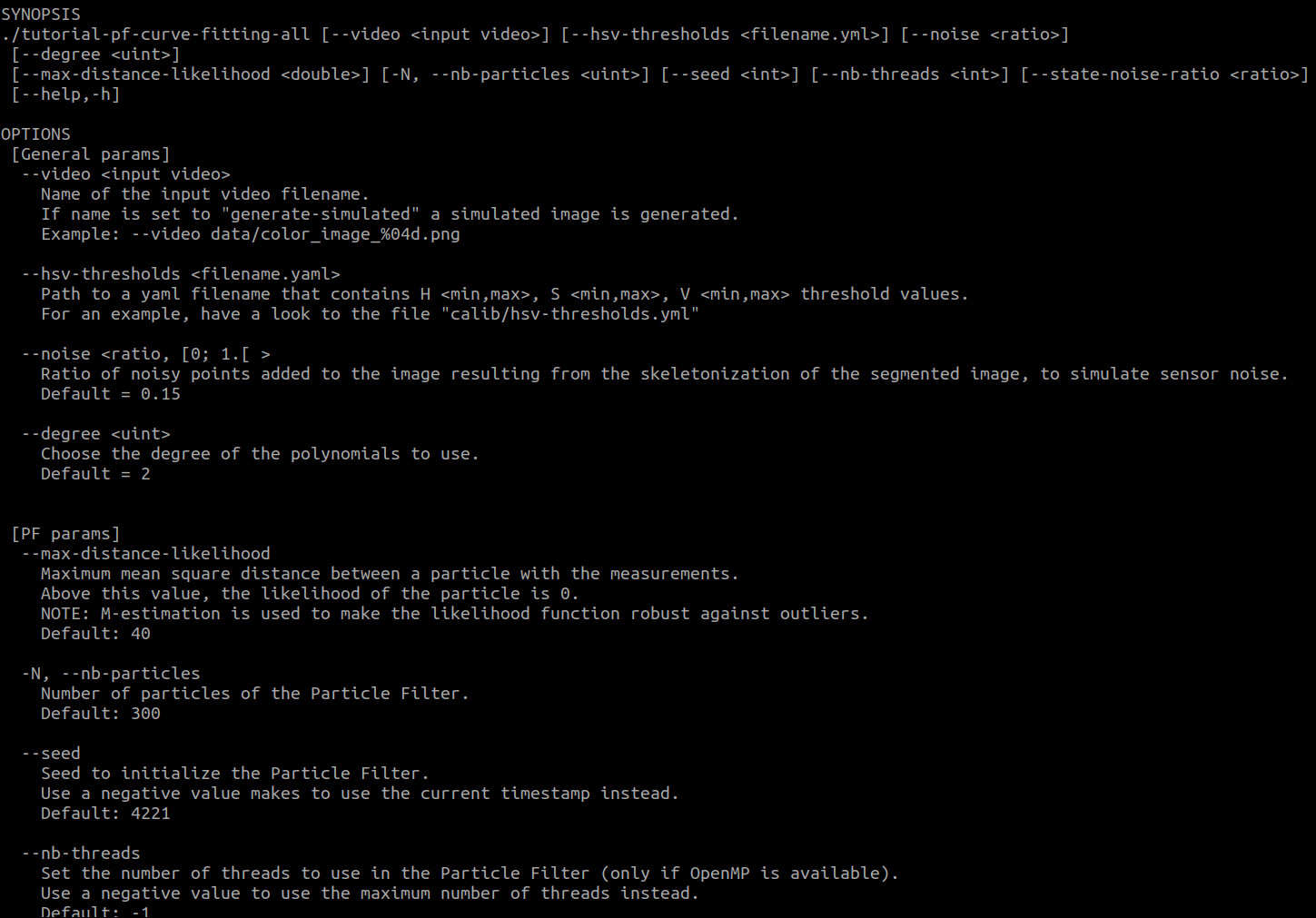
Screenshot of the tutorial Graphical User Interface

For the tutorial-pf-curve-fitting-pf.cpp and tutorial-pf-curve-fitting-all.cpp tutorials, the PF must be initialized. You are asked if you would rather use a manual initialization (left click) or an automatic one (right click).

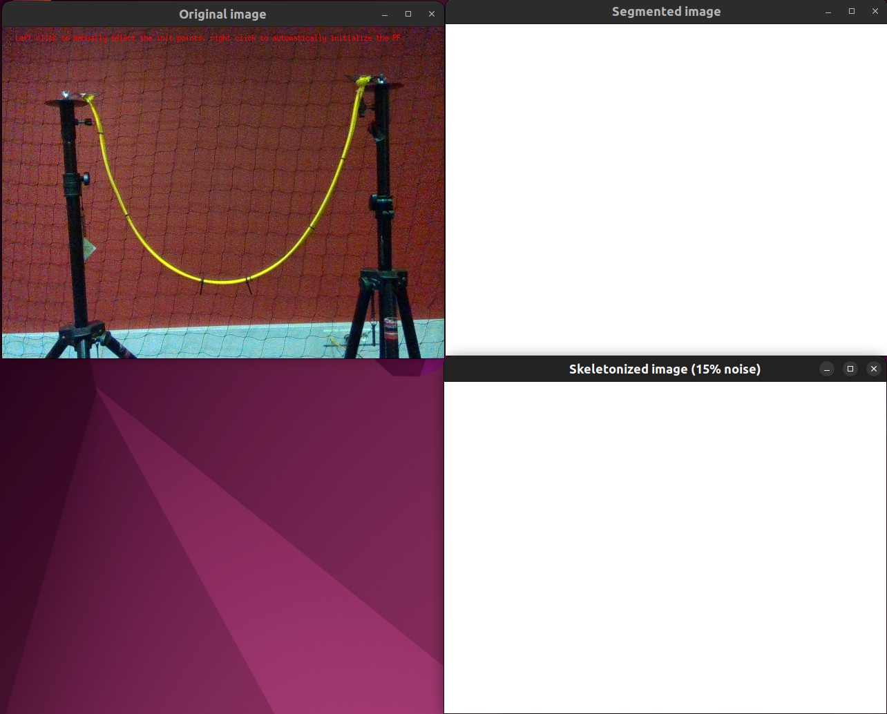
Screenshot of the tutorial initialization step

Then, for all the tutorials, you can either display the images one-by-one (left click) or automatically switch from an image to the next one (middle click). You can leave the program whenever you want using a right click.

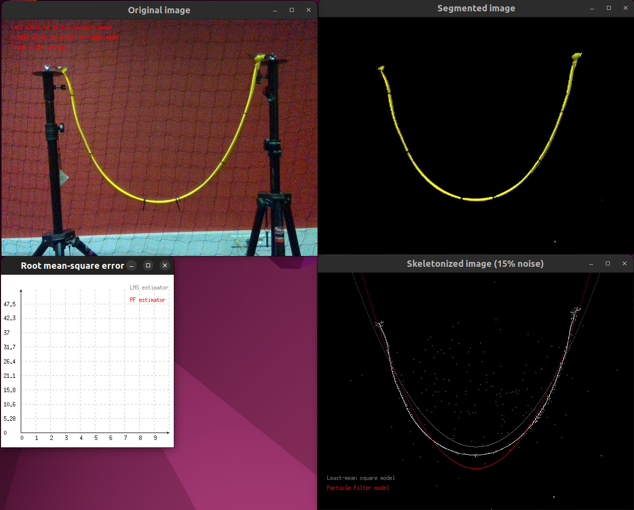
Screenshot of the tutorial during its run step

General explanations about the tutorials

Notes about the segmentation and skeletonization of the image

The segmentation of the image using HSV encoding has been presented in the Tutorial: HSV low/high range tuner tool .

A calibration file containing the segmentation parameters for the default sequence can be found in the calib folder. If you want to use your own sequence, please run the tutorial-hsv-range-tuner.cpp tutorial to extract the parameters that correspond to your own sequence and edit the file calib/hsv-thresholds.yml .

The skeletonization of the segmented image is not the topic of this tutorial. Thus, we invite the interested readers to read by themselves the corresponding method in the vpTutoSegmentation.cpp file.

Explanations about the Particle Filter

The internal state of the PF contains the coefficients of the interpolation polynomial. Be $v(u) = \sum_{i=0}^N a_i u^i$ the interpolation polynomial whose highest degree is N. The internal state of the PF is of size N + 1 such as:

$\begin{array}{lcl} \textbf{x}[i] &=& a_i \end{array}$

The measurement $\textbf{z}$ corresponds to the vector of vpImagePoint that forms the skeletonized version of the segmented image. Be and the horizontal and vertical pixel coordinates of the $i^{th}$ marker. The measurement vector can be written as:

$\begin{array}{lcl} \textbf{z}[i] &=& vpImagePoint(v_i , u_i) \end{array}$

Explanations about the Least-Mean Square method

The Least-Mean Square method is a standard method to solve a polynomial interpolation problem. The polynomial interpolation problem can be written in matrices form as follow:

$\begin{array}{llcl} & \textbf{A}\textbf{x} &=& \textbf{b} \\ \iff & \textbf{X} &=& \textbf{A}^+\textbf{b} \\ \end{array}$

where $\textbf{A}^+$ denotes the Moore-Penrose pseudo-inverse of the matrix A, with:

$\begin{array}{lcl} \textbf{A}[i][j] &=& u_i^j \end{array} \\ \begin{array}{lcl} \textbf{x}[i] &=& a_i \end{array} \\ \begin{array}{lcl} \textbf{b}[i] &=& v_i \end{array}$

Important note: due to numerical unstability, the pixel coordinates cannot be used directly in the Least-Mean square method. Indeed, using pixel coordinates leads to having an ill-conditionned $\textbf{A}$ matrix. Consequently, in all the tutorials, the pixel coordinates are normalized by dividing them by the height and width of the image before running any interpolation.

Detailed explanations about the tutorials

We will now present the different tutorials and explained their important parts.

Details on the tutorial-pf-curve-fitting-lms.cpp

This tutorial goal is to show how a Least-Mean Square method can be used to perform polynomial interpolation and the impact of noise on such technique.

To visualize the accuracy of the method, a vpPlot is instantiated in the following part of the code:

#ifdef VISP_HAVE_DISPLAY
  unsigned int plotHeight = 350, plotWidth = 350;
  int plotXpos = static_cast<int>(data.m_legendOffset.get_u());
  int plotYpos = static_cast<int>(data.m_I_orig.getHeight() + 4. * data.m_legendOffset.get_v());
  vpPlot plot(1, plotHeight, plotWidth, plotXpos, plotYpos, "Root mean-square error");
  plot.initGraph(0, 1);
  plot.setLegend(0, 0, "LMS estimator");
  plot.setColor(0, 0, vpColor::gray);
#endif

At each iteration, the new frame is read, then segmented and skeletonized in the following section of code:

    std::cout << "Iter " << nbIter << std::endl;
    data.m_grabber.acquire(data.m_I_orig);
 
    // Perform color segmentation
    tutorial::performSegmentationHSV(data);
 
    std::vector<vpImagePoint> edgePoints = tutorial::extractSkeleton(data);
 
    std::vector<vpImagePoint> noisyEdgePoints = tutorial::addSaltAndPepperNoise(edgePoints, data);

The method addSaltAndPepperNoise permits to add a user-defined percentage of salt-and-pepper noise, to evaluate the robustness of the method against noise.

The polynomial interpolation is performed in the following section of the code:

lmsFitter.fit(noisyEdgePoints);

It relies on the following method of the vpTutoMeanSquareFitting class:

void vpTutoMeanSquareFitting::fit(const std::vector<vpImagePoint> &pts)
{
  vpMatrix A; // The matrix that contains the u^i
  vpMatrix X; // The matrix we want to estimate, that contains the polynomial coefficients.
  vpMatrix b; // The matrix that contains the v values
 
  // Fill the matrices that form the system we want to solve
  vpTutoParabolaModel::fillSystem(m_degree, m_height, m_width, pts, A, b);
 
  // Compute the parabola coefficients using the least-mean-square method.
  X = A.pseudoInverse() * b;
  m_model = vpTutoParabolaModel(X, m_height, m_width);
  m_isFitted = true;
}

The matrices that form the system that needs to be solved are filled in the vpTutoParabolaModel class (we remind the reader that normalization of the pixel coordinates is performed to avoid numerical unstability):

  static void fillSystem(const unsigned int &degree, const double &height, const double &width, const std::vector<VISP_NAMESPACE_ADDRESSING vpImagePoint> &pts, VISP_NAMESPACE_ADDRESSING vpMatrix &A, VISP_NAMESPACE_ADDRESSING vpMatrix &b)
  {
    const unsigned int nbPts = static_cast<unsigned int>(pts.size());
    const unsigned int nbCoeffs = degree + 1;
    std::vector<VISP_NAMESPACE_ADDRESSING vpImagePoint> normalizedPts;
    // Normalization to avoid numerical instability
    for (const auto &pt: pts) {
      normalizedPts.push_back(VISP_NAMESPACE_ADDRESSING vpImagePoint(pt.get_i() / height, pt.get_j() / width));
    }
    A.resize(nbPts, nbCoeffs, 1.); // Contains the u^i
    b.resize(nbPts, 1); // Contains the v coordinates
    for (unsigned int i = 0; i < nbPts; ++i) {
      double u = normalizedPts[i].get_u();
      double v = normalizedPts[i].get_v();
      for (unsigned int j = 0; j < nbCoeffs; ++j) {
        A[i][j] = std::pow(u, j);
      }
      b[i][0] = v;
    }
  }

Details on the tutorial-pf-curve-fitting-pf.cpp

This tutorial is meant to show how a Particle Filter could be used to model a wire thanks to polynomial interpolation.

To initialize a Particle Filter, a guess of the initial state must be given to it. The more accurate is the initial guess, the quicker the PF will converge. The initialization can be done either manually or automatically thanks to the following piece of code:

 
std::vector<vpImagePoint> automaticInitialization(tutorial::vpTutoCommonData &data)
{
  // Initialization-related variables
  const unsigned int minNbPts = data.m_degree + 1;
  const unsigned int nbPtsToUse = 10 * minNbPts;
  std::vector<vpImagePoint> initPoints;
 
  // Perform HSV segmentation
  tutorial::performSegmentationHSV(data);
 
  // Extracting the skeleton of the mask
  std::vector<vpImagePoint> edgePoints = tutorial::extractSkeleton(data);
  unsigned int nbEdgePoints = static_cast<unsigned int>(edgePoints.size());
 
  if (nbEdgePoints < nbPtsToUse) {
    return edgePoints;
  }
 
  // Uniformly extract init points
  auto ptHasLowerU = [](const vpImagePoint &ptA, const vpImagePoint &ptB) {
    return ptA.get_u() < ptB.get_u();
    };
  std::sort(edgePoints.begin(), edgePoints.end(), ptHasLowerU);
 
  unsigned int idStart, idStop;
  if (nbEdgePoints > nbPtsToUse + 20) {
    // Avoid extreme points in case it's noise
    idStart = 10;
    idStop = static_cast<unsigned int>(edgePoints.size()) - 10;
  }
  else {
    // We need to take all the points because we don't have enough
    idStart = 0;
    idStop = static_cast<unsigned int>(edgePoints.size());
  }
 
  // Sample uniformly the points starting from the left of the image to the right
  unsigned int sizeWindow = idStop - idStart + 1;
  unsigned int step = sizeWindow / (nbPtsToUse - 1);
  for (unsigned int id = idStart; id <= idStop; id += step) {
    initPoints.push_back(edgePoints[id]);
  }
  return initPoints;
}
 
std::vector<vpImagePoint> manualInitialization(const tutorial::vpTutoCommonData &data)
{
  // Interaction variables
  const bool waitForClick = true;
  vpImagePoint ipClick;
  vpMouseButton::vpMouseButtonType button;
 
  // Display variables
  const unsigned int sizeCross = 10;
  const unsigned int thicknessCross = 2;
  const vpColor colorCross = vpColor::red;
 
  // Initialization-related variables
  const unsigned int minNbPts = data.m_degree + 1;
  std::vector<vpImagePoint> initPoints;
 
  bool notEnoughPoints = true;
  while (notEnoughPoints) {
    // Initial display of the images
    vpDisplay::display(data.m_I_orig);
 
    // Display the how-to
    vpDisplay::displayText(data.m_I_orig, data.m_ipLegend, "Left click to add init point (min.: " + std::to_string(minNbPts) + "), right click to estimate the initial coefficients of the Particle Filter.", data.m_colorLegend);
    vpDisplay::displayText(data.m_I_orig, data.m_ipLegend + data.m_legendOffset, "A middle click reinitialize the list of init points.", data.m_colorLegend);
    vpDisplay::displayText(data.m_I_orig, data.m_ipLegend + data.m_legendOffset + data.m_legendOffset, "If not enough points have been selected, a right click has no effect.", data.m_colorLegend);
 
    // Display the already selected points
    unsigned int nbInitPoints = static_cast<unsigned int>(initPoints.size());
    for (unsigned int i = 0; i < nbInitPoints; ++i) {
      vpDisplay::displayCross(data.m_I_orig, initPoints[i], sizeCross, colorCross, thicknessCross);
    }
 
    // Update the display
    vpDisplay::flush(data.m_I_orig);
 
    // Get the user input
    vpDisplay::getClick(data.m_I_orig, ipClick, button, waitForClick);
 
    // Either add the clicked point to the list of initial points or stop the loop if enough points are available
    switch (button) {
    case vpMouseButton::vpMouseButtonType::button1:
      initPoints.push_back(ipClick);
      break;
    case vpMouseButton::vpMouseButtonType::button2:
      initPoints.clear();
      break;
    case vpMouseButton::vpMouseButtonType::button3:
      (initPoints.size() >= minNbPts ? notEnoughPoints = false : notEnoughPoints = true);
      break;
    default:
      break;
    }
  }
 
  return initPoints;
}
 
vpColVector computeInitialGuess(tutorial::vpTutoCommonData &data)
{
  // Vector that contains the init points
  std::vector<vpImagePoint> initPoints;
 
#ifdef VISP_HAVE_DISPLAY
  // Interaction variables
  const bool waitForClick = true;
  vpImagePoint ipClick;
  vpMouseButton::vpMouseButtonType button;
 
  // Display variables
  const unsigned int sizeCross = 10;
  const unsigned int thicknessCross = 2;
  const vpColor colorCross = vpColor::red;
 
  bool automaticInit = false;
 
  // Initial display of the images
  vpDisplay::display(data.m_I_orig);
  vpDisplay::displayText(data.m_I_orig, data.m_ipLegend, "Left click to manually select the init points, right click to automatically initialize the PF", data.m_colorLegend);
 
  // Update the display
  vpDisplay::flush(data.m_I_orig);
 
  // Get the user input
  vpDisplay::getClick(data.m_I_orig, ipClick, button, waitForClick);
 
  // Either use the automatic initialization or the manual one depending on the user input
  switch (button) {
  case vpMouseButton::vpMouseButtonType::button1:
    automaticInit = false;
    break;
  case vpMouseButton::vpMouseButtonType::button3:
    automaticInit = true;
    break;
  default:
    break;
  }
 
  if (automaticInit) {
    // Get automatically the init points from the segmented image
    initPoints = tutorial::automaticInitialization(data);
  }
  else {
    // Get manually the init points from the original image
    initPoints = tutorial::manualInitialization(data);
  }
 
#else
  // Get the init points from the segmented image
  initPoints = tutorial::automaticInitialization(data);
#endif
 
  // Compute the coefficients of the parabola using Least-Mean-Square minimization.
  tutorial::vpTutoMeanSquareFitting lmsFitter(data.m_degree, data.m_I_orig.getHeight(), data.m_I_orig.getWidth());
  lmsFitter.fit(initPoints);
  vpColVector X0 = lmsFitter.getCoeffs();
  std::cout << "---[Initial fit]---" << std::endl;
  std::cout << lmsFitter.getModel();
  std::cout << "---[Initial fit]---" << std::endl;
 
  // Display info about the initialization
  vpDisplay::display(data.m_I_orig);
  vpDisplay::displayText(data.m_I_orig, data.m_ipLegend, "Here are the points selected for the initialization.", data.m_colorLegend);
  unsigned int nbInitPoints = static_cast<unsigned int>(initPoints.size());
  for (unsigned int i = 0; i < nbInitPoints; ++i) {
    const vpImagePoint &ip = initPoints[i];
    vpDisplay::displayCross(data.m_I_orig, ip, sizeCross, colorCross, thicknessCross);
  }
 
  // Update display and wait for click
  lmsFitter.display(data.m_I_orig, vpColor::red, static_cast<unsigned int>(data.m_ipLegend.get_v() + 2 * data.m_legendOffset.get_v()), static_cast<unsigned int>(data.m_ipLegend.get_u()));
  vpDisplay::displayText(data.m_I_orig, data.m_ipLegend + data.m_legendOffset, "A click to continue.", data.m_colorLegend);
  vpDisplay::flush(data.m_I_orig);
  vpDisplay::getClick(data.m_I_orig, waitForClick);
 
  return X0;
}

A Particle Filter needs a function to evaluate the likelihood of a particle. We decided to use a Gaussian-based function that penalizes particles whose polynomial model has a Root Mean Square Error with regard to the measurement points greater than a given threshold. To be robust against outliers, we use the Tukey M-estimator. The likelihood function is implemented in a functor to be able to pass additional information such as the height and width of the input image:

class vpTutoLikelihoodFunctor
{
public:
  vpTutoLikelihoodFunctor(const double &stdev, const unsigned int &height, const unsigned int &width)
    : m_height(height)
    , m_width(width)
  {
    double sigmaDistanceSquared = stdev * stdev;
    m_constantDenominator = 1. / std::sqrt(2. * M_PI * sigmaDistanceSquared);
    m_constantExpDenominator = -1. / (2. * sigmaDistanceSquared);
  }
 
 
  double likelihood(const vpColVector &coeffs, const std::vector<vpImagePoint> &meas)
  {
    double likelihood = 0.;
    unsigned int nbPoints = static_cast<unsigned int>(meas.size());
 
    // Generate a model from the coefficients stored in the particle state
    vpTutoParabolaModel model(coeffs, m_height, m_width);
 
    // Compute the residual between each measurement point and its equivalent in the model
    vpColVector residuals(nbPoints);
    for (unsigned int i = 0; i < nbPoints; ++i) {
      double squareError = tutorial::evaluate(meas[i], model);
      residuals[i] = squareError;
    }
 
    // Use Tukey M-estimator to be robust against outliers
    vpRobust Mestimator;
    vpColVector w(nbPoints, 1.);
    Mestimator.MEstimator(vpRobust::TUKEY, residuals, w);
    double sumError = w.hadamard(residuals).sum();
 
    // Compute the likelihood as a Gaussian function
    likelihood = std::exp(m_constantExpDenominator * sumError / w.sum()) * m_constantDenominator;
    likelihood = std::min(likelihood, 1.0); // Clamp to have likelihood <= 1.
    likelihood = std::max(likelihood, 0.); // Clamp to have likelihood >= 0.
    return likelihood;
  }
private:
  double m_constantDenominator; 
  double m_constantExpDenominator; 
  unsigned int m_height; 
  unsigned int m_width; 
};

This likelihood functor compute the residuals using the following evaluation functions:

 
double evaluate(const vpImagePoint &pt, const vpTutoParabolaModel &model)
{
  double u = pt.get_u();
  double v = pt.get_v();
  double v_model = model.eval(u);
  double error = v - v_model;
  double squareError = error * error;
  return squareError;
}
 
double evaluate(const vpColVector &coeffs, const unsigned int &height, const unsigned int &width, const std::vector<vpImagePoint> &pts)
{
  unsigned int nbPts = static_cast<unsigned int>(pts.size());
  vpColVector residuals(nbPts);
  vpColVector weights(nbPts, 1.);
  vpTutoParabolaModel model(coeffs, height, width);
  // Compute the residuals
  for (unsigned int i = 0; i < nbPts; ++i) {
    double squareError = evaluate(pts[i], model);
    residuals[i] = squareError;
  }
  double meanSquareError = residuals.sum() / static_cast<double>(nbPts);
  return std::sqrt(meanSquareError);
}

A Particle Filter needs to perform a weighted average to compute the filtered state. Performing a weighted average of the particles polynomial coefficients would not lead to satisfying results, as it is not mathematically correct. Instead, we decided to generate a given number of "control points" by each particle. The number of control points generated by a particle is dictated by its associated weight. Then, we compute the polynomial coefficients that best fit all these control points using a Least-Square minimization technique. The weighted average is performed thanks to the following functor:

class vpTutoAverageFunctor
{
public:
  vpTutoAverageFunctor(const unsigned int &degree, const unsigned int &height, const unsigned int &width)
    : m_degree(degree)
    , m_height(height)
    , m_width(width)
  { }
 
  vpColVector averagePolynomials(const std::vector<vpColVector> &particles, const std::vector<double> &weights, const vpParticleFilter<std::vector<vpImagePoint>>::vpStateAddFunction &)
  {
    const unsigned int nbParticles = static_cast<unsigned int>(particles.size());
    const double nbParticlesAsDOuble = static_cast<double>(nbParticles);
    // Compute the sum of the weights to be able to determine the "importance" of a particle with regard to the whole set
    const double sumWeight = std::accumulate(weights.begin(), weights.end(), 0.);
 
    // Defining the total number of control points we want to generate
    const double nbPointsForAverage = 10. * nbParticlesAsDOuble;
    std::vector<vpImagePoint> initPoints;
 
    // Creating control points by each particle
    for (unsigned int i = 0; i < nbParticles; ++i) {
      // The number of control points a particle can generate is proportional to the ratio of its weight w.r.t. the sum of the weights
      double nbPoints = std::floor(weights[i] * nbPointsForAverage / sumWeight);
      if (nbPoints > 1.) {
        // The particle has a weight high enough to deserve more than one points
        vpTutoParabolaModel curve(particles[i], m_height, m_width);
        double widthAsDouble = static_cast<double>(m_width);
        // Uniform sampling of the control points along the polynomial model
        double step = widthAsDouble / (nbPoints - 1.);
        for (double u = 0.; u < widthAsDouble; u += step) {
          double v = curve.eval(u);
          vpImagePoint pt(v, u);
          initPoints.push_back(pt);
        }
      }
      else if (nbPoints == 1.) {
        // The weight of the particle make it have only one control point
        // We sample it at the middle of the image
        vpTutoParabolaModel curve(particles[i], m_height, m_width);
        double u = static_cast<double>(m_width) / 2.;
        double v = curve.eval(u);
        vpImagePoint pt(v, u);
        initPoints.push_back(pt);
      }
    }
    // We use Least-Mean Square minimization to compute the polynomial model that best fits all the control points
    vpTutoMeanSquareFitting lms(m_degree, m_height, m_width);
    lms.fit(initPoints);
    return lms.getCoeffs();
  }
 
private:
  unsigned int m_degree; 
  unsigned int m_height; 
  unsigned int m_width; 
};

A Particle Filter needs a process function to project the particles forward in time. For this scenario, we decided to use the identity, and let the randomness of the Particle Filter manage the potential motion of the wire.

vpColVector fx(const vpColVector &coeffs, const double &/*dt*/)
{
  vpColVector updatedCoeffs = coeffs; // We use a constant position model
  return updatedCoeffs;
}

The initialization parameters of the Particle Filter are defined in the following section of code:

  const double maxDistanceForLikelihood = data.m_pfMaxDistanceForLikelihood; // The maximum allowed distance between a particle and the measurement, leading to a likelihood equal to 0..
  const double sigmaLikelihood = maxDistanceForLikelihood / 3.; // The standard deviation of likelihood function.
  const unsigned int nbParticles = data.m_pfN; // Number of particles to use
  std::vector<double> stdevsPF; // Standard deviation for each state component
  for (unsigned int i = 0; i < data.m_degree + 1; ++i) {
    double ampliMax = data.m_pfRatiosAmpliMax[i] * X0[i];
    stdevsPF.push_back(ampliMax / 3.);
  }
  unsigned long seedPF; // Seed for the random generators of the PF
  const float period = 33.3f; // 33.3ms i.e. 30Hz
  if (data.m_pfSeed < 0) {
    seedPF = static_cast<unsigned long>(vpTime::measureTimeMicros());
  }
  else {
    seedPF = data.m_pfSeed;
  }
  const int nbThread = data.m_pfNbThreads;

The initialization functions of the Particle Filter are defined in the following section of code:

  vpParticleFilter<std::vector<vpImagePoint>>::vpProcessFunction processFunc = tutorial::fx;
  tutorial::vpTutoLikelihoodFunctor likelihoodFtor(sigmaLikelihood, data.m_I_orig.getHeight(), data.m_I_orig.getWidth());
  using std::placeholders::_1;
  using std::placeholders::_2;
  vpParticleFilter<std::vector<vpImagePoint>>::vpLikelihoodFunction likelihoodFunc = std::bind(&tutorial::vpTutoLikelihoodFunctor::likelihood, &likelihoodFtor, _1, _2);
  vpParticleFilter<std::vector<vpImagePoint>>::vpResamplingConditionFunction checkResamplingFunc = vpParticleFilter<std::vector<vpImagePoint>>::simpleResamplingCheck;
  vpParticleFilter<std::vector<vpImagePoint>>::vpResamplingFunction resamplingFunc = vpParticleFilter<std::vector<vpImagePoint>>::simpleImportanceResampling;
  tutorial::vpTutoAverageFunctor averageCpter(data.m_degree, data.m_I_orig.getHeight(), data.m_I_orig.getWidth());
  using std::placeholders::_3;
  vpParticleFilter<std::vector<vpImagePoint>>::vpFilterFunction meanFunc = std::bind(&tutorial::vpTutoAverageFunctor::averagePolynomials, &averageCpter, _1, _2, _3);

The Particle Filter is then constructed thanks to the following lines:

  // Initialize the PF
  vpParticleFilter<std::vector<vpImagePoint>> filter(nbParticles, stdevsPF, seedPF, nbThread);
  filter.init(X0, processFunc, likelihoodFunc, checkResamplingFunc, resamplingFunc, meanFunc);

Finally, the filtering is performed thanks to the following line:

filter.filter(noisyEdgePoints, period);

The filtered state is retrieve thanks to the following line:

vpColVector Xest = filter.computeFilteredState();

Details on the tutorial-pf-curve-fitting-all.cpp

The tutorial-pf-curve-fitting-all.cpp reuse what has already been presented in the Details on the tutorial-pf-curve-fitting-lms.cpp and Details on the tutorial-pf-curve-fitting-pf.cpp sections.

Its main objective is to compare the time performances and robustness against noise of the two methods. The ratio of noise can be set using the Command Line Interface using the –noise option. For instance,

$ ./tutorial-pf-curve-fitting-all --video data/color_image_0%03d.png --noise <ratio in the intervall [0.; 1.[>

will add 50% of noisy pixels to the skeletonized image.

You can experiment by varying this parameter (and others as well) to see the impact on the different methods. With 15% noisy pixels and more, the Particle Filter tends to have a greater accuracy than the LMS method, but it takes more times to run.

Table of Contents