Introduction

This tutorial gives some hints to boost your visual servo control law in order to speed up the time to convergence.

Note that all the material (source code and image) described in this tutorial is part of ViSP source code and could be downloaded using the following command:

$ svn export https://github.com/lagadic/visp.git/trunk/tutorial/visual-servoing/ibvs

To illustrate this tutorial let us consider the example tutorial-ibvs-4pts-plotter.cpp introduced in Tutorial: Image-based visual servo. This example consider an image based visual servoing using four points as visual features.

In the general case, considering $\dot {\bf q}$ as the input velocities to the robot controller, the control laws provided in vpServo class lead to the following control law $\dot {\bf q} = \pm \lambda {{\bf \widehat J}_e}^+ {\bf e}$ where the sign is negative for an eye in hand servo and positive for an eye to hand servo, $\lambda$ is a constant gain, ${\bf \widehat J}_e$ is the task Jacobian and $\bf e$ is the error to regulate to zero. As described in [2], this control law ensure an exponential decoupled decrease of the error ${\dot {\bf e}} = \pm \lambda {\bf e}$ .

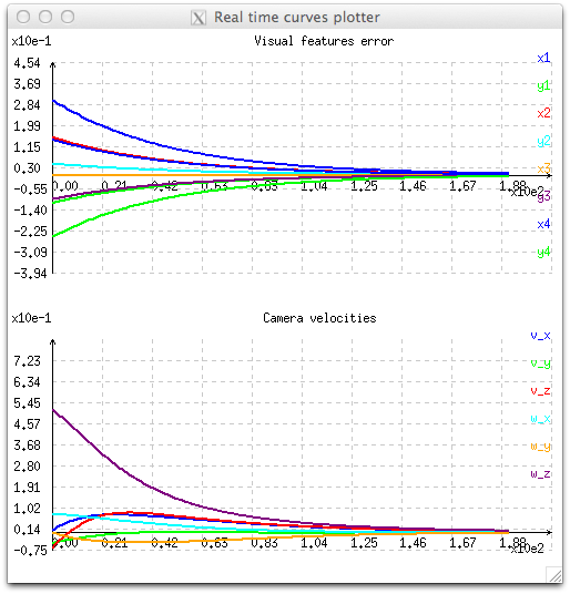
This behavior is illustrated with the next figure, where we see the exponential decrease of the eight visual features (x and y for each point) and the corresponding six velocities that are applied to the robot controller. As a consequence, velocities are high when the error is important, and very low when the error is small near the convergence. At the beginning, we can also notice velocity discontinuities with velocities varying from zero to high values in one iteration.

Convergence in 191 iterations with a constant gain.

This behavior can be reproduced running tutorial-ibvs-4pts-plotter.cpp example. Here after we recall the important lines of code used to compute the control law:

vpServo task ;
task.setServo(vpServo::EYEINHAND_CAMERA);
task.setInteractionMatrixType(vpServo::CURRENT);
task.setLambda(0.5);                              // Set the constant gain value
for (unsigned int i = 0 ; i < 4 ; i++) {
  ...
  task.addFeature(p[i], pd[i]);                   // Add visual features to the task
}
while(1) {
  for (unsigned int i = 0 ; i < 4 ; i++) {
    ...
    vpFeatureBuilder::create(p[i], point[i]);     // Update the visual features used in the task
  }
  vpColVector v = task.computeControlLaw();       // Compute the control law
}

Using an adaptive gain

As implemented in tutorial-ibvs-4pts-plotter-gain-adaptive.cpp it is possible to adapt the gain $\lambda$ in order to depend on the infinity norm of the task Jacobian. The usage of an adaptive gain rather than a constant gain allows to reduce the convergence time. In that case the gain becomes:

$\lambda (x) = a * exp (-b*x) + c$

where $ a $ , $ b $ and $ c $ are constant parameters and $ x $ is the infinity norm of the task Jacobian to consider.

The parameters $a,b,c$ are not set directly. They are computed from three other parameters $\lambda(0), \lambda(\infty), {\dot \lambda}(0)$ that are more intuitive to tune:

$a = \lambda(0) - \lambda(\infty)$

$b = {\dot \lambda}(0) / a$

$c = \lambda(\infty)$

Here $\lambda(0)$ represents the gain when $x=0$ , $\lambda(\infty)$ represents the gain when $x=\infty$ and ${\dot \lambda}(0)$ represents the slope of $\lambda(x)$ when $x=0$ .

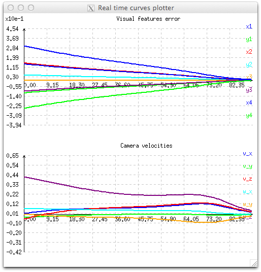
The impact of the adaptive gain is illustrated in the next figure. During the servo, velocities applied to the controller are higher, especially when the visual error ${\bf e}$ is small. But as in the previous section, using an adaptive gain doesn't insure continuous velocities especially at the first iteration.

Convergence in 91 iterations with an adaptive gain.

This behavior can be reproduced running tutorial-ibvs-4pts-plotter-gain-adaptive.cpp example. Compared to the previous code given in Introduction and available in tutorial-ibvs-4pts-plotter.cpp, here after we give the new lines of code that were introduced to use an adaptive gain:

vpAdaptiveGain lambda(4, 0.4, 30); // lambda(0)=4, lambda(oo)=0.4 and lambda_dot(0)=30

task.setLambda(lambda);

Continuous sequencing

As implemented in tutorial-ibvs-4pts-plotter-continuous-gain-adaptive.cpp it is also possible to ensure continuous sequencing to avoid velocity discontinuities. This behavior is achieved by introducing an additional term to the general form of the control law. This additional term comes from the task sequencing approach described in [21] equation (17). It allows to compute continuous velocities by avoiding abrupt changes in the command.

The form of the control law considered here is the following:

${\bf \dot q} = \pm \lambda {{\bf \widehat J}_e}^+ {\bf e} \mp \lambda {{\bf \widehat J}_{e(0)}}^+ {{\bf e}(0)} \exp(-\mu t)$

where :

${\bf \dot q}$ is the resulting continuous velocity command to apply to the robot controller.
the sign of the control law depends on the eye in hand or eye to hand configuration.
$\bf J$ is the Jacobian of the task.
$\bf e = (s-s^*)$ is the error to regulate.
is the time.
$\mu$ is a gain. We recommend to set this value to 4.
${\bf \widehat J}_{e(0)}^+ {\bf e}(0)$ is the value of ${\bf \widehat J}_e^+ {\bf e}$ when .

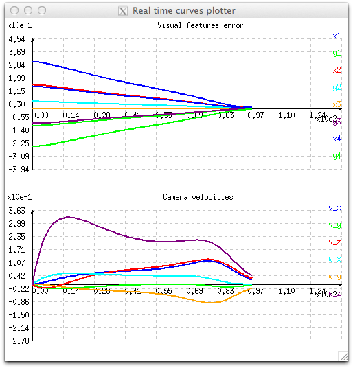
The effect of continuous sequencing is illustrated in the next figure where during the first iterations velocities are starting from zero.

Convergence in 98 iterations with an adaptive gain and continuous sequencing.

This behavior can be reproduced running tutorial-ibvs-4pts-plotter-continuous-gain-adaptive.cpp example. Compared to the previous code given in Using an adaptive gain and available in tutorial-ibvs-4pts-plotter-gain-adaptive.cpp, here after we give the new line of code that were introduced to ensure continuous sequencing:

vpColVector v = task.computeControlLaw(iter*robot.getSamplingTime());

Table of Contents

Introduction

Using an adaptive gain

Continuous sequencing