Introduction

In this tutorial, we will show how to generate synthetic data that can be used to train a neural network, thanks to blenderproc.

Most of the (manual) work when training a neural network resides in acquiring and labelling data. This process can be slow, tedious and error prone. A solution to avoid this step is to use synthetic data, generated by a simulator/computer program. This approach comes with multiple advantages:

Data acquisition is fast
It is easy to acquire accurate ground truth labels
Variations in the training data can be easily added

There are however, some drawbacks:

More knowledge of the scene is required: in the case of detection, we require a 3D model of the object, which is not the case for true images
A difference between simulated and real data can be apparent and negatively impact network performance (this is called the Sim2Real gap)

The latter point is heavily dependent on the quality of the generated images and the more realistic the images, the better the expected results.

Blender, using ray tracing, can generate realistic images. To perform data generation, Blenderproc has been developed and is an extremely useful and flexible tool to generate realistic scenes from Python code.

Along with RGB images, Blenderproc can generate different labels or inputs:

Depth map
Normals
Semantic segmentation
Instance segmentation
Bounding box
Optical flow (not provided in our generation script)

In this tutorial, we will install blenderproc and use it to generate simple but varied scenes containing objects of interest. We provide a simple, object-centric generation script that should suffice in many cases. However, since Blenderproc is easy to use, with many examples included in the documentation, readapting this script to your needs should be easy.

Requirements

First, you should start by installing blenderproc. First, start by creating a new conda environment to avoid potential conflicts with other Python packages.

$ conda create --name blenderproc python=3.10 pip
$ conda activate blenderproc
$ pip install blenderproc

Note: Our generation script has been tested with blenderproc 2.5.0 (with Blender 3.3 under the hood) and python 3.10.

You can then run the Blenderproc sample example with:

(blenderproc) $ blenderproc quickstart

This may take some time, as Blenderproc downloads its own version of Blender and sets up its own environment. This setup will only be performed once.

Once Blenderproc is done, you can check its output with:

(blenderproc) $ blenderproc vis hdf5 output/0.hdf5

Blenderproc stores its output in HDF5 file format. Each HDF5 may contain the RGB image, along with depth, normals, and other modalities.

For the simulator to provide useful data, we should obtain a set of realistic textures (thus helping close the Sim2Real gap). Thankfully, Blenderproc provides a helpful script to download a dataset of materials from cc0textures.com, containing more than 1500 high resolution materials. To download the materials, run

(blenderproc) $ blenderproc download cc_textures path/to/folder/where/to/save/materials

Warning: Because the materials are in high definition, downloading the full dataset may take a large amount of disk space (30+ GB). If this is too much for you, you can safely delete some of the materials or stop the script after it has acquired enough materials. While using a small number of materials can be useful when performing quick tests, using the full set should be preferred as variety helps when transferring your deep learning model to real world data.

Running the object-centric generation script

We will now run the generation script. The script places a random set of objects in a simple cubic room, with added distractors. Materials of the walls and distractors are randomized.

This script and an example configuration file can be found in the script/dataset_generator folder of your ViSP source directory.

The basic algorithm is:

For each scene:
  Choose N target objects from the provided models
  Add noise to the N objects (material properties, size, geometry)
  Generate a scene:
    - compute s = length of the larget diagonal of the axis-aligned bounding box of the largest object
    - set room_size = s * random_scale_factor
    - Create the ground, walls and ceiling of the room (with size room_size) and select a random material for each of them
    - Add random distractors, sampled from spheres, cubes, cylinders and monkey heads (Suzanne)
    For each distractor:
      - Sample a random position and orientation in the room
      - Select a random material from cc0
      - Add noise to PBR
      - Potentially add displacement
      - Potentially set distractor as emissive (emitting light)
    - Add random lights, either point lights or spots
    For each light:
      - Sample a random intensity and position
      - Sample a random color
      - If the light is a spot, orient it so that it focuses on a target object
    If simulating physics:
      - Simulate physics for a fixed time and set final object poses
    Remove objects that left the room (Physics collisions)
  Sample camera poses:
    For each sample to generate:
      Do while camera pose is not correct:
        - Select a target object
        - Select a point of interest in the bounding box of the object
        - Sample a random camera location in a clamped ball around the object
          - Camera position is set to have a minimum/maximum distance to the point of interest that is dependent on the object size
        - Set camera orientation to look at the point of interest, with a random rotation around the optical axis
        - Camera pose is correct if target object is visible and camera does not clip through an object or a wall
  - Call blender rendering
  - Save data in HDF5 format
    - If required, compute occlusion-aware bounding boxes
    - If required, save object pose in camera frame

Many randomization parameters can be modified to alter the rendering, as explained in Generation configuration.

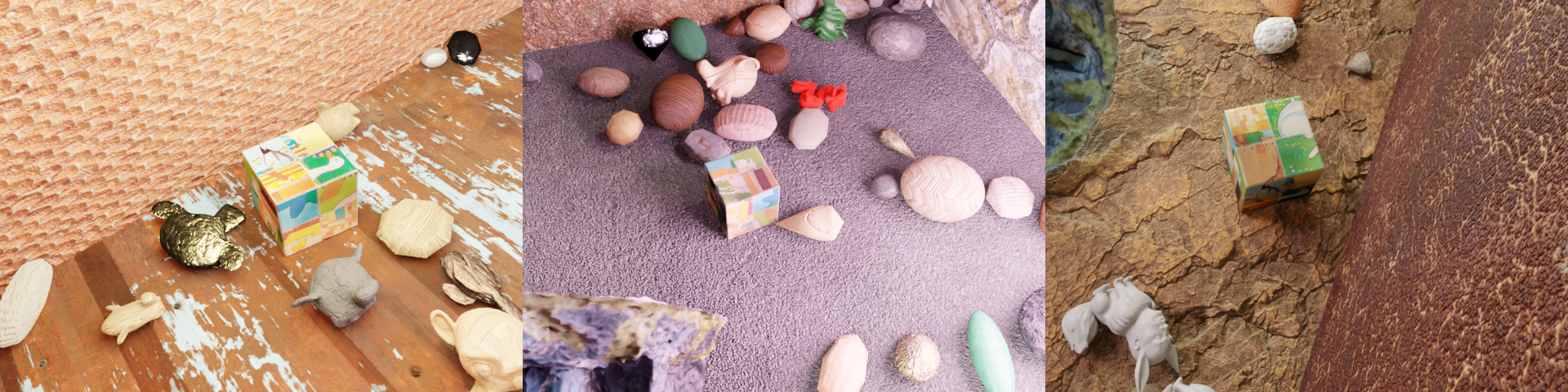
With this simple approach, we can obtain images such as:

3D model format

To use this data generation tool, you should first provide the 3D models. You can provide multiple models, which will be sampled randomly during generation.

The models should be contained in a folder as such:

- models
  - objectA
    - model.obj
    - model.mtl
    - texture.png
  - objectB
    - another_model.obj
    - another_model.mtl

When setting up the configuration file in Generation configuration, "models_path" should point to the root folder, models. Each subfolder should contain a single object, in .obj format (with potential materials and textures). Each object will be considered as having its own class, the class name being the name of the subfolder (e.g., objectA or objectB). The class indices start with 1, and are sorted alphabetically depending on the name of the class (e.g., objectA = 1, objectB = 2).

Generation configuration

Configuring the dataset generation is done through a JSON file. An example configuration file can be seen below:

{
  "numpy_seed": 19,
  "blenderproc_seed": "69",
 
  "models_path": "./megapose-models",
  "cc_textures_path": "./cc0",
  "camera": {
    "px": 600,
    "py": 600,
    "u0": 320,
    "v0": 240,
    "h": 480,
    "w": 640,
    "randomize_params_percent": 5.0
  },
  "rendering": {
    "max_num_samples": 32,
    "denoiser": "OPTIX"
  },
  "scene": {
    "room_size_multiplier_min": 5.0,
    "room_size_multiplier_max": 10.0,
    "simulate_physics": false,
    "max_num_textures": 50,
    "distractors": {
      "min_count": 20,
      "max_count": 50,
      "min_size_rel_scene": 0.05,
      "max_size_rel_scene": 0.1,
      "custom_distractors": "./megapose-distractors",
      "custom_distractor_proba": 0.5,
      "displacement_max_amount": 0.0,
      "pbr_noise": 0.5,
      "emissive_prob": 0.0,
      "emissive_min_strength": 2.0,
      "emissive_max_strength": 5.0
    },
    "lights": {
      "min_count": 3,
      "max_count": 6,
      "min_intensity": 50,
      "max_intensity": 200
    },
    "objects": {
      "min_count": 2,
      "max_count": 5,
      "multiple_occurences": true,
      "scale_noise": 0.2,
      "displacement_max_amount": 0.0,
      "pbr_noise": 0.3,
      "cam_min_dist_rel": 1.0,
      "cam_max_dist_rel": 3.0
    }
  },
  "dataset": {
    "save_path": "./output_blenderproc",
    "scenes_per_run": 1,
    "num_scenes": 100,
    "images_per_scene": 10,
    "empty_images_per_scene": 2,
    "pose": true,
    "depth": false,
    "normals": false,
    "segmentation": false,
    "detection": true,
    "detection_params": {
      "min_side_size_px": 10,
      "min_visibility_percentage": 0.3,
      "points_sampling_occlusion": 100
    }
  }
}

The general parameters are:

Name	Type, possible values	Description
numpy_seed	Int	Seed for numpy's random functions. Allows for reproducible results.
blenderproc_seed	String	Seed for Blenderproc. Allows for reproducible results.
models_path	String	Path to the folder containing the models. See 3D model format
cc_textures_path	String	Path to the folder containing the CC0 materials.

You can also control some of the rendering parameters. This will impact the rendering time and the quality of the generated RGB images. These parameters are located in the "rendering" field.

Name	Type, possible values	Description
max_num_samples	Int > 0	Number of rays per pixels. A lower number results in noisier images (especially in scenes with large variations).
denoiser	One of [null, "INTEL", "OPTIX"]	Which denoiser to use after performing ray tracing. null indicates that no denoiser is used. "OPTIX" requires a compatible Nvidia GPU. Using a denoiser allows to obtain a clean image, with a low number of rays per pixels.

You can also modify the camera's intrinsic parameters. The camera uses an undistorted perspective projection model. For more information on camera parameters, see vpCameraParameters. These parameters are found in the "camera" field of the configuration.

Name	Type, possible values	Description
px	Float	See vpCameraParameters
py	Float	See vpCameraParameters
v0	Float	See vpCameraParameters
u0	Float	See vpCameraParameters
h	Int	Height of the generated images.
w	Int	Width of the generated images.
randomize_params_percent	Float, [0, 100)	Controls the randomization of the camera parameters 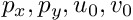. If randomize_params_percent > 0, then, each time a scene is created the intrinsics are perturbed around the given values. For example, if this parameters is equal to 0.10 and , then the used when generating images will be in the range [450, 550].

To customize the scene, you can change the parameters in the "scene" field:

Name	Type, possible values	Description
room_size_multiplier_min	Float > 1.0, < room_size_multiplier_max	Minimum room size as a factor of the biggest sampled target object. The room is cubic. The size of the biggest object is the length of the largest diagonal of its axis-aligned bounding box. This tends to overestimate the size of the object. If the size of the biggest object is 0.5m, room_size_multiplier_max = 2 and room_size_multiplier_max = 4, then the room's size will be randomly sampled to be between 1m and 2m.
room_size_multiplier_max	Float > room_size_multiplier_min	Minimum room size as a factor of the biggest sampled target object. The room is cubic. The size of the biggest object is the length of the largest diagonal of its axis-aligned bounding box. This tends to overestimate the size of the object. If the size of the biggest object is 0.5m, room_size_multiplier_max = 2 and room_size_multiplier_max = 4, then the room's size will be randomly sampled to be between 1m and 2m.
simulate_physics	Boolean	Whether to simulate physics. If false, then objects will be floating across the room. If true, then objects will fall to the ground.
max_num_textures	Int > 0	Max number of textures per blenderproc run. If scenes_per_run is 1, max_num_textures = 50 and the number of distractors is more than 50, then the 50 textures will be used across all distractors (and walls). In this case, new materials will be sampled for each scene.
distractors	Dictionary	See below
lights	Dictionary	See below
objects	Dictionary	See below

Distractors are small, simple objects that are added along with the target objects to create some variations and occlusions. You can also load custom objects as distractors. To modify their properties, you can change the "distractors" field of the scene

Name	Type, possible values	Description
min_count	Int >= 0, < max_count	Minimum number of distractors to place in the room.
max_count	Int > min_count	Maximum number of distractors to place in the room.
custom_distractors	string, or null	If not null, path to a folder containing custom distractor objects, in .obj or .ply format.
custom_distractor_proba	float, >= 0.0, <= 1.0	If custom_distractors is not null, probability that a distractor is sampled from the user specified distractors.
min_size_rel_scene	Float > 0.0	Minimum size of the distractors, relative to the room size. If the room size is 0.5m and min_size_rel_scene = 0.1, then the minimum size of distractor will be 0.05m. Scale is applied independently on each axis.
max_size_rel_scene	Float < 1.0, > min_size_rel_scene	maximum size of the distractors, relative to the room size. If the room size is 0.5m and max_size_rel_scene = 0.2, then the maximum size of distractor will be 0.1m. Scale is applied independently on each axis.
displacement_max_amount	Float >= 0.0	Amount of displacement to apply to distractors. Displacement subdivides the mesh and displaces each of the distractor's vertices according to a random noise pattern. This option greatly slows down rendering: set it to 0 if needed.
pbr_noise	Float >= 0.0	Amount of noise to add to the material properties of the distractors. These properties include the specularity, the "metallicness" and the roughness of the material, according to Blender's principled BSDF.
emissive_prob	Float >= 0.0 , <= 1.0	Probability that a distractor becomes a light source: its surface emits light. Set to more than 0 to add more light variations and shadows.
emissive_min_strength	Float >= 0.0, < emissive_max_strength	Minimum emission strength for a distractor that emits lights. In Watts/m².
emissive_max_strength	Float > emissive_min_strength	Maxmimum emission strength for a distractor that emits lights. In Watts/m².

To change the lighting behaviour, see the options below:

Name	Type, possible values	Description
min_count	Int >= 0, < max_count	Minimum number of lights in the scene.
max_count	Int > min_count	Maximum number of lights in the scene
min_intensity	Float > 0.0, < max_intensity	Minimum intensity of a light. In Watts.
max_intensity	Float > min_intensity	Maximum intensity of a light. In Watts.

To change the sampling behaviour of target objects, see the properties below:

Name	Type, possible values	Description
min_count	Int >= 0, < max_count	Minimum number of target objects in the scene.
max_count	Int > min_count	Maximum number of target objects in the scene.
multiple_occurences	Boolean	Whether a single object can appear multiple times in the same scene (sampling with replacement).
scale_noise	Float >= 0.0	Object size noise. if scale_noise > 0.0, the object is scaled uniformly on all axes (it does not appear stretched)
displacement_max_amount	Float >= 0.0	Amount of displacement to apply to target objects. Displacement subdivides the mesh and displaces each of the distractor's vertices according to a random noise pattern. This option greatly slows down rendering: set it to 0 if needed. Note that this is in absolute units: and does not vary depending on the size of the object.
pbr_noise	Float >= 0.0	Amount of noise to add to the material properties of the target objects. These properties include the specularity, the "metallicness" and the roughness of the material, according to Blender's principled BSDF.
cam_min_dist_rel	Float >= 0.0, < cam_max_dist_rel	Minimum distance of the camera to the point of interest of the object when sampling camera poses. This is expressed in terms of the size of the target object. If the target object has a size of 0.5m and cam_min_dist_rel = 1.5, then the closest possible camera will be at 0.75m away from the point of interest.
cam_max_dist_rel	Float >= cam_min_dist_rel	Maximum distance of the camera to the point of interest of the object when sampling camera poses. This is expressed in terms of the size of the target object. If the target object has a size of 0.5m and cam_max_dist_rel = 2.0, then the farthest possible camera will be 1m away from the point of interest.

Finally, we can customize the dataset that we will generate from the given scenes. This includes the number of scenes, images, and what information to save.

All the data will be stored in HDF5 format, which can then be unpacked later.

To customize the dataset, modify the options in the "dataset" field:

Name	Type, possible values	Description
save_path	String	Path to the folder that will contain the final dataset. This folder will contain one folder per scene, and each sample of a scene will be its own HDF5 file.
scenes_per_run	Int > 0	Number of scenes to generate per blenderproc run. Between blenderproc runs, Blender is restarted in order to avoid memory issues.
num_scenes	Int > 0	Total number of scenes to generate. Generating many scenes will add more diversity to the dataset as object placement, materials and lighting are randomized once per scene.
images_per_scene	Int > 0	Number of images to generate per scene. The total number of samples in the dataset will be num_scenes * (images_per_scene + empty_images_per_scene).
empty_images_per_scene	Int >= 0, <= images_per_scene	Number of images without target objects to generate per scene. The camera poses for these images are sampled from the poses used to generate images with target objects. Thus, the only difference will be that the objects are not present, the rest of the scene is left untouched.
pose	Boolean	Whether to save the pose of target objects that are visible in the camera. The pose of the objects are expressed in the camera frame as an homogeneous matrix $^{c}\mathbf{T}_{o}$
depth	Boolean	Whether to save the depth buffer associated to the RGB image. Same size as the RGB image.
normals	Boolean	Whether to save the normal map associated to the RGB image. Same size as the RGB image. The normals are 3D unit vectors, expressed in the camera frame.
segmentation	Boolean	Whether to save the segmentation maps (by class and by instance). Segmentation by class only contains the target objects (class >= 1). Segmentation by instance includes every visible object.
detection	Boolean	Whether to save the bounding box detections. In this case, bounding boxes are not computed from the segmentation map (also possible with Blenderproc), but rather in way such that occlusion does not influence the final bounding box. The detections can be filtered with the parameters in "detection_params".
detection_params:min_size_size_px	Int >= 0	Minimum side length of a detection for it to be considered as valid. Used to filter really far or small objects, for which detection would be hard.
detection_params:min_visibility	Float [0.0, 1.0]	Percentage of the object that must be visible for a detection to be considered as valid. The visibility score is computed as such: First, the vertices of the mesh that are behind the camera are filtered. Then, the vertices that are outside of the camera's field of view are filtered. Then, we randomly sample "detection_params:points_sampling_occlusion" points to test whether the object is occluded (test done through ray casting). If too many points are filtered, then the object is considered as not visible and detection is invalid.

Running the script to generate data

Once you have configured the generation to your liking, navigate to the script/dataset_generator located in your ViSP source directory.

You can then run the generate_dataset.py script as such

(blenderproc) user@machine:~/visp/script/dataset_generator $ python generate_dataset.py --config path/to/config.json

If all is well setup, then the dataset generation should start and run.

Warning: If during generation, you encounter a message about invalid camera placement, try to make room_size_multiplier_min and room_size_multiplier_max larger, so that more space is available for object placement.

To give an idea of generation time, generating 1000 images (with a resolution of 640 x 480) and detections of a single object, with a few added distractors, takes around 30mins on a Quadro RTX 6000.

Once generation is finished, you are ready to leverage the data to train your neural network.

Using and parsing the generation output

The dataset generated by Blender is located in the "dataset:save_path" path that you specified in your JSON configuration file.

The dataset has the following structure

- dataset
  - 0
    - 0.hdf5
    - 1.hdf5
    - ...
  - 1
    - 0.hdf5
    - 1.hdf5
    - ...
  - ...
  - classes.txt

There is one subfolder per scene, and each HDF5 file is a single sample that may contain RGB, depth, normals, etc.

You can visualise the generated images (RGB, depth, normals, segmentation maps) by running

(blenderproc) $ blenderproc vis hdf5 path/to/your/output/0/*.hdf5

You will then see something that looks like this, depending on the outputs that you chose in the configuration file:

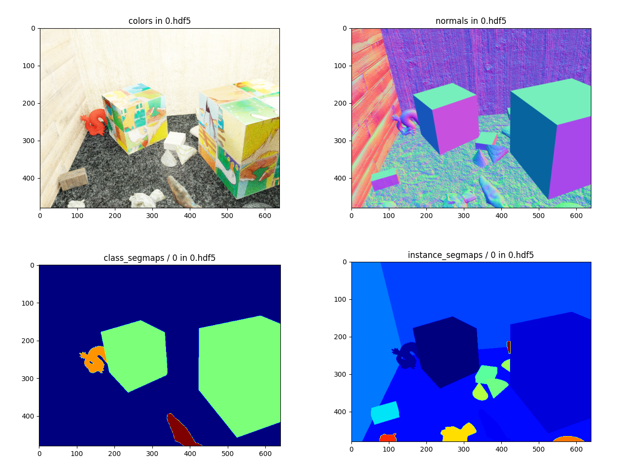
where you can replace the "0" in the path with another number, which corresponds to the generated scene index. You can also specify the path to a single HDF5 file to view one sample at a time.

Using detections to finetune a YoloV7

To help, we provide a script that reformats a blenderproc dataset to the format expected by YoloV7. This script can be run like this:

(blenderproc) $ python export_for_yolov7.py --input path/to/dataset --output path/to/yolodataset --train-split 0.8

here "--input" indicates the path to the location of the blenderproc dataset, while "--output" points to the folder where the dataset in the format that YoloV7 expects will be saved. "--train-split" is an argument that indicates how much of the dataset is kept for training. A value of 0.8 indicates that 80% of the dataset is used for training, while 20% is used for validation. The split is performed randomly across all scenes (a scene may be visible in both train and validation sets).

Once the script has run, the folder "path/to/yolodataset" should be created and contain the dataset as expected by YoloV7. This folder contains a "dataset.yml" file, which will be used when training a YoloV7. It contains: the following:

names:
- esa
nc: 1
train: /local/user/yolov7_esa_dataset/images/train
val: /local/user/yolov7_esa_dataset/images/val

where nc is the number of class, "names" are the class names, and "train" and "val" are the paths to the dataset splits.

To start training a YoloV7, you should download the repository and install the required dependencies. Again, we will create a conda environment. You can also use a docker container, as explained in the documentation. We also download the pretrained yolo model, that we will finetune on our own dataset.

~ $ git clone https://github.com/WongKinYiu/yolov7.git
~ $ cd yolov7
~/yolov7 $ conda create --name yolov7 pip
~/yolov7 $ conda activate yolov7
(yolov7) ~/yolov7 $ pip install -r requirements.txt
(yolov7) ~/yolov7 $ wget https://github.com/WongKinYiu/yolov7/releases/download/v0.1/yolov7-tiny.pt

To fine-tune a YoloV7, we should create two new files: the network configuration and the hyperparameters. We will reuse the ones provided for the tiny model.

CFG=cfg/training/yolov7-tiny-custom.yaml
cp cfg/training/yolov7-tiny.yaml $CFG
 
HYP=data/hyp.scratch.custom.yaml
cp data/hyp.scratch.tiny.yaml $HYP

Next open the new cfg file, and modify the number of classes (set "nc" from 80 to the number classes you have in your dataset).

You can also modify the hyperparameters file to add more augmentation during training.

To fine-tune the YoloV7-tiny on our data, run

YOLO_DATASET=/path/to/dataset
IMG_SIZE=640
YOLO_NAME=blenderproc-tiny
python train.py --workers 8 --device 0 --batch-size 64 --data "${YOLO_DATASET}/dataset.yaml" --img $IMG_SIZE $IMG_SIZE --cfg $CFG --weights yolov7-tiny.pt --name  $YOLO_NAME --hyp $HYP

Note that if your run fine-tuning multiple times, then a number will be appended to the name that you have given to your model.

If you run out of memory during training, change the batch size to a lower value.

Here is an overview of the generated images and the resulting detections for a simple model (cube) and a NeRF-reconstructed one:

Parsing HDF5 with a custom script

In Python, an HDF5 file can be read like a dictionary.

With the following script, you can inspect the content of an HDF5 file:

from pathlib import Path
import numpy as np
import h5py
import json
 
if __name__ == '__main__':
  dataset_path = Path('output')
  for scene_folder in dataset_path.iterdir():
    if not scene_folder.is_dir():
      continue
    print(f'Reading scene {scene_folder.name}')
    for sample in scene_folder.iterdir():
      if not sample.name.endswith('.hdf5'):
          continue
      print(f'\tReading sample {sample.name}')
      with h5py.File(sample) as f:
          # Image data
          keys = ['colors', 'depth', 'normals', 'class_segmaps', 'instance_segmaps']
          for key in keys:
             if key in f:
                data = np.array(f[key])
                print(f'\t\t{key}: shape = {data.shape}, type = {data.dtype}')
          # Json objects
          if 'instance_attribute_maps' in f:
            print('\t\tMapping between instance and class:')
            text = np.array(f['instance_attribute_maps']).tobytes()
            json_rep = json.loads(text)
            print(json_rep)
            print()
 
          if 'object_data' in f:
            text = np.array(f['object_data']).tobytes()
            json_rep = json.loads(text)
 
            for object_idx, object_data in enumerate(json_rep):
              print(f'\t\tObject {object_idx} data: ')
              for obj_k in object_data.keys():
                print(f'\t\t\t{obj_k} = {object_data[obj_k]}')
              print()

Running on a custom dataset with all outputs enabled (see Generation configuration) we obtain the following output:

...
Reading scene 4
  Reading sample 0.hdf5
    colors: shape = (480, 640, 3), type = uint8
    depth: shape = (480, 640), type = float32
    normals: shape = (480, 640, 3), type = float32
    class_segmaps: shape = (480, 640), type = uint8
    instance_segmaps: shape = (480, 640), type = uint8
    Mapping between instance and class:
      [{'idx': 5, 'category_id': 2}, {'idx': 7, 'category_id': 3}, {'idx': 10, 'category_id': 0}, {'idx': 11, 'category_id': 0},
       {'idx': 14, 'category_id': 0}, {'idx': 18, 'category_id': 0}, {'idx': 22, 'category_id': 0}, {'idx': 32, 'category_id': 0},
       {'idx': 37, 'category_id': 0}]

    Object 0 data:
      class = 2
      name = cube.001
      cTo = [[-0.9067991971969604, -0.12124679982662201, 0.40374961495399475, 0.06561152129493264],
            [-0.399792343378067, 0.5511342883110046, -0.7324047088623047, 0.31461843930247957],
            [-0.1337185800075531, -0.8255603313446045, -0.548241913318634, 0.01648345626311576],
            [0.0, 0.0, 0.0, 1.0]]
      bounding_box = [138.9861569133729, 254.62236838239235, 100.20349472431002, 107.79005297420909]

    Object 1 data:
      class = 3
      name = dragon.002
      cTo = [[-0.9067991971969604, -0.12124679982662201, 0.40374961495399475, 0.06561152129493264],
             [-0.399792343378067, 0.5511342883110046, -0.7324047088623047, 0.31461843930247957],
             [-0.1337185800075531, -0.8255603313446045, -0.548241913318634, 0.01648345626311576],
             [0.0, 0.0, 0.0, 1.0]]
      bounding_box = [314.54058632091767, 202.86607727119753, 70.64506150004479, 90.54480823214647]
...

Both depth and normals are represented as floating points, conserving accuracy.
The object data is represented as a JSON document. Which you can directly save or reparse to save only the information of interest.
Object poses are expressed in the camera frame and are represented as homogeneous matrix.
Bounding boxes coordinates are in pixels, and the values are [x_min, y_min, width, height]

You can modify this script to export the dataset to another format, as it was done in Using detections to finetune a YoloV7.

Next steps

If you use this generator to train a detection network, you can combine it with Megapose to perform 6D pose estimation and tracking. See Tutorial: Tracking with MegaPose.

Table of Contents