Tutorial: IBVS with Panda 7-dof robot from Franka Emika

Table of Contents

• Introduction
• Image-based visual servoing
• Next tutorial

Introduction

This tutorial explains how to do an image-based visual-servoing with the Panda 7-dof robot from Franka Emika equipped with an Intel Realsense SR300 camera. It follows Tutorial: PBVS with Panda 7-dof robot from Franka Emika that explains also how to setup the robot.

Image-based visual servoing

At this point we suppose that you follow all the Prerequisites given in Tutorial: PBVS with Panda 7-dof robot from Franka Emika.

An example of image-based visual servoing using Panda robot equipped with a Realsense camera is available in servoFrankaIBVS.cpp.

• Attach your Realsense camera to the robot end-effector
• Put an Apriltag in the camera field of view
• If not already done, follow Tutorial: Camera extrinsic calibration to estimate the homogeneous transformation between robot end-effector and camera frame. We suppose here that the file is located in tutorial/calibration/eMc.yaml.

Now enter in example/servo-franka folder and run servoFrankaIBVS binary using --eMc to locate the file containing the transformation. Other options are available. Using --help show them:

$ cd example/servo-franka
$ ./servoFrankaIBVS --help
./servoFrankaIBVS [--ip <default 192.168.1.1>] [--tag_size <marker size in meter; default 0.12>] [--eMc <eMc extrinsic file>] [--quad_decimate <decimation; default 2>] [--adaptive_gain] [--plot] [--task_sequencing] [--no-convergence-threshold] [--verbose] [--help] [-h]

Run the binary activating the plot and using a constant gain:

$ ./servoFrankaIBVS --eMc ../../tutorial/calibration/eMc.yaml --plot

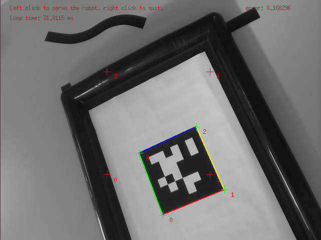
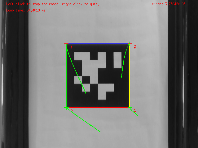
Use the left mouse click to enable the robot controller, and the right click to quit the binary.

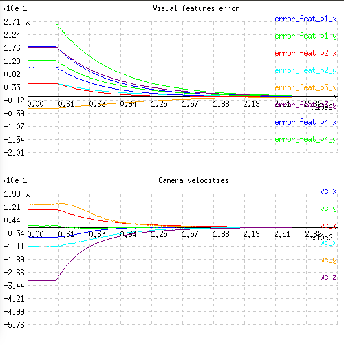
At this point the behaviour that you should observe is the following:

Legend: Example of initial position. The goal is here to center the 4 tag corners in the image.

Legend: Example of final position reached after position-based visual servoing. In green, you can see the trajectories in the image of the tag corners. When the camera extrinsic parameters are well estimated these trajectories are straight lines.

Legend: Corresponding visual-features (x and y coordinates of the corner points in the image plane) and velocities applied to the robot in the camera frame. You can observe an exponential decrease of the visual features.

You can also activate an adaptive gain that will make the convergence faster:

$ ./servoFrankaIBVS --eMc ../../tutorial/calibration/eMc.yaml --plot --adaptive_gain

You can also start the robot with a zero velocity at the beginning introducing task sequencing option:

$ ./servoFrankaIBVS --eMc ../../tutorial/calibration/eMc.yaml --plot --task_sequencing

And finally you can activate the adaptive gain and task sequencing:

$ ./servoFrankaIBVS --eMc ../../tutorial/calibration/eMc.yaml --plot --adaptive_gain --task_sequencing

To learn more about adaptive gain and task sequencing see Tutorial: How to boost your visual servo control law.

Next tutorial

You are now ready follow Tutorial: Image-based visual servo that will give some hints on image-based visual servoing in simulation with a free flying camera.